


Introduction
The response of the Antarctic ice sheet to climate change is a principal unknown in determining potential sea-level rise (Reference Church and StockerChurch and others, 2013; Reference StockerIPCC, 2013). There is an emerging consensus that the mass balance of the Antarctic ice sheet is now negative (Reference Vaughan and StockerVaughan and others, 2013), but uncertainty remains in the magnitude and causes of this trend. Only prolonged time series of relevant observations can resolve these uncertainties (Reference Wouters, Bamber, Van den Broeke, Lenaerts and SasgenWouters and others, 2013), and only detailed observations of ice thickness, surface elevation and basal boundary conditions, tied to better-constrained models of ice physics, will allow predictions of future mass change to be made. In particular, the East Antarctic ice sheet (EAIS) contribution to sea-level rise is poorly constrained (Reference Vaughan and StockerVaughan and others, 2013), due to sparse ice-thickness measurements and limited coverage of surface-elevation change data along its remote 8000 km long margin.
Altimetry of the ice-sheet surface provides a powerful constraint on ice-sheet mass balance and behavior. Incoherent orbital radar altimeters (e.g. Envisat (Reference Flament, Berthier and RémyFlament and others, 2014)), which are not interrupted by cloud cover, yield long time series and have the capacity to provide great coverage of coastal Antarctica; however, they have limited horizontal resolution (a few kilometers) and strong sensitivity to surface slopes. Coherent orbital radar altimetry, currently represented by CryoSat-2 (Reference McMillanMcMillan and others, 2014; Reference Siegfried, Fricker, Roberts, Scambos and TulaczykSiegfried and others, 2014), can improve footprint resolution to less than 0.5 km × 1.5 km. However, issues of variable surface penetration remain. In contrast, orbital and airborne laser altimeters offer smaller footprint sizes restricted to the surface interface. The single-beam Geoscience Laser Altimeter System (GLAS), on board the Ice, Cloud and land Elevation Satellite (ICESat; Reference Schutz, Zwally, Shuman, Hancock and DiMarzioSchutz and others, 2005) operated between 2003 and 2009, with footprints ∼80 m wide separated by 175 m. ICESat repeated a pattern of orbital tracks up to 15 times over its 6 year lifetime, to retrieve high-resolution records of surface elevation change. However, ICESat suffered pointing errors of up to hundreds of meters in the cross-track direction, and these errors complicate the interpretation of repeat-track elevation change where significant cross-track slopes are present.
A follow-on mission for ICESat, ICESat-2, will address the cross-track problem using multiple pairs of fixed beams spaced by 90 m on the ground; in order to deploy these multiple beams, a new low-power lidar technology, photon counting (Reference DegnanDegnan, 2002), will be deployed on ICESat-2’s Advanced Topographic Laser Altimeter System (ATLAS). To continue the time series between ICESat and the expected 2017 launch of ICESat-2, NASA initiated the Operation IceBridge airborne program to conduct repeated altimetry observations of key regions. As part of this program, the International Collaborative Exploration of the Cryosphere by Airborne Profiling (ICECAP) consortium collected a 3 year surface-elevation dataset acquired over East Antarctica using an advanced airborne scanning photon-counting lidar (PCL), coupled to a legacy nadir-pointing laser profiler (here called the LAS).
ICECAP systematically targeted high-leverage ICESat tracks for re-flight to extend the surface-elevation record, in particular for tracks where clouds had interrupted the ICESat record. We use the well-characterized LAS system to provide profile measurements of surface elevation, in tandem with the PCL (which has higher absolute range uncertainties) which provides cross-track slope information for correction of ICESat observations. Together the LAS and PCL form the Airborne Laser Altimeter with Mapping Optics (ALAMO).
We first describe the context for surface-elevation change in this region, including the existing ICESat record. We then describe the LAS and PCL components of the altimetry system and its operation, using the example of the 2011 ICECAP field season (ICP4). We discuss our approach for the generation of data products to address the Operation IceBridge science goals. We then extend our coverage to all three years of field campaigns, and focus on three key sites along the Indo-Pacific margin of East Antarctica.
The 2003–09 ICESat Observation Record
After its launch in 2003, ICESat conducted seventeen 33 day campaigns of altimetry observations, which have led to numerous discoveries about the mass balance and sub-glacial hydrology of the Antarctic ice sheet (Reference ThomasThomas and others, 2004; Reference Fricker, Scambos, Bindschadler and PadmanFricker and others, 2007; Reference Pritchard, Arthern, Vaughan and EdwardsPritchard and others, 2009, Reference Pritchard, Ligtenberg, Fricker, Vaughan, Van den Broeke and Padman2012; Reference Smith, Fricker, Joughin and TulaczykSmith and others, 2009). Elevation changes extracted included the discrete surface-elevation change between distinct observations, Δz/Δt, and the mean secular trend in elevation change, dz/dt. These campaigns repeatedly targeted 696 orbital tracks, approximately evenly spaced around the continent. Given the low density of inter-orbit crossovers near much of the coast of Antarctica, a goal of the mission was to accurately retrieve elevation change at high resolution along each track.
The GLAS instrument was a single-beam, high-power, 1064 nm laser system that illuminated a ∼64 m wide footprint on the ground per pulse (Reference AbshireAbshire and others, 2005). Pulses were collected at 40 Hz, with 176 m between footprints. Tracks were repeated with an accuracy of ±60 m (1 standard deviation) either side of the reference track, meaning that cross-track slopes of 0.1° could induce apparent changes in surface elevation of ±10 cm. Assuming a planar surface slope, ten repeated ICESat tracks allow definitive separation of slope and change effects (Reference Smith, Fricker, Joughin and TulaczykSmith and others, 2009; Reference AbdalatiAbdalati and others, 2010; Reference ZwallyZwally and others, 2011); however, in coastal areas, cloud cover reduced the number of tracks with data. For this study, we used the GLAH12 Release 633 product (Reference ZwallyZwally and others, 2012), with a subsequent ‘Gaussian-centroid’ correction to the data applied (Reference ZwallyZwally, 2013; Reference Borsa, Moholdt, Fricker and BruntBorsa and others, 2014).
ICESat dz/dt determination
To provide context for our results we determined average long-term surface-elevation change rates using ICESat data alone, using a planar-fit based method. Other approaches (polynomial fits (Reference ZwallyZwally and others, 2011) and triangulated irregular networks (Reference Pritchard, Arthern, Vaughan and EdwardsPritchard and others, 2009)) have been used to derive elevation change from the ICESat record; we elect to use the planar-fit method for the simplicity of its assumptions and similarity to the approach we used for the ALAMO data analysis. Best-fit planes are fitted to the ICESat data in 700 m long bins every 500 m along track, and dz/dt is obtained using a least-squares method. Input data are filtered by cross-track distance. We output residuals and estimate 95% confidence intervals using a χ 2 distribution assumption.
The 2010–12 Airborne Observation Record in East Antarctica
A critical element of Operation IceBridge is airborne altimetry, and several platforms have been used: Goddard Space Flight Center’s Airborne Topographic Mapper (ATM; Reference KrabillKrabill and others, 2002; Reference MartinMartin and others, 2012) and Land, Vegetation and Ice Sensor (LVIS; Reference Blair, Rabine and HoftonBlair and others, 1999) and the University of Texas at Austin’s ALAMO, fielded as an element of ICECAP. ALAMO has been fielded over one Greenland and three Antarctic field seasons, and represents one of the few civilian operational scanning PCL systems.
Operation IceBridge adopted the altimetry science requirements (Operation IceBridge Science Definition Team, 2012) of measuring annual changes in glacier, icecap and ice-sheet surface elevation sufficiently accurately to detect 0.15 m changes in uncrevassed and 1.0 m changes in crevassed regions along sampled profiles over distances of 500 m, and measuring Antarctic surface elevation along established airborne altimeter and ICESat underflight lines that extend from near the glacier margin to near the ice divide. The data products discussed in this paper are intended to satisfy these requirements.
Field operations
ICECAP used a long-range ski-equipped DC-3T modified for aerogeophysics by the University of Texas, and equipped with ice-penetrating radar, gravimeter, magnetometers and laser altimeters to investigate the geometry (Reference RobertsRoberts and others, 2011), long-term history (Reference YoungYoung and others, 2011), stratigraphy (Reference CavitteCavitte, 2011) and subglacial hydrology (Reference WrightWright and others, 2012) of the East Antarctic ice sheet. An important goal of ICECAP is to extend the record of ice-sheet surface-elevation change, a proxy for ice-volume change and, hence, sea-level change. The aircraft operated from McMurdo Station (MCM), Dumont d’Urville Station (DDU) and Casey Station (CSY). The three field seasons relevant to this paper took place in 2010/11 (ICP3), November–December 2011 (ICP4) and November– December 2012 (ICP5).
The ICECAP geophysical system was installed on the aircraft at the McMurdo seasonal sea-ice runway at the start of each field season. Installation was followed by a calibration flight involving multiple crossovers over flat ice. On typical data-collection flights, the aircraft was flown 600–1000 m above the ground, at a ground speed of 90 m s−1. Approximately 100 GB of range data were acquired per 6 hour flight.
As part of Operation IceBridge, ICECAP flew grids over Mulloch Glacier, David Glacier, McMurdo Ice Shelf, Totten Glacier, Moscow University Ice Shelf and Dome C, as well as several ICESat tracks in the Totten Glacier, David Glacier and Byrd Glacier catchments (Fig. 1). ICECAP also re-flew three ICESat tracks over the unnamed tributary ice streams of the Cook Ice Shelf, which lie in George V Land overlying deep troughs extending into the Wilkes Subglacial Basin.

Fig. 1. Locations of geolocated ALAMO surface recoveries (Reference Blankenship, Kempf, Young and LindzeyBlankenship and others, 2013a) in the Indo-Pacific sector of East Antarctica. Background is bed elevations, showing major subglacial basins (Reference FretwellFretwell and others, 2013). Outlined regions are box a: McMurdo Ice Shelf (Fig. 4); box b: the George V Coast; and box c: Dome C (target for calibration in Fig. 5). Major glaciers and ice shelves mentioned in the text are noted, with ICESat tracks discussed in this text indicated in dark blue. MCM: McMurdo Station; DDU: Dumont d’Urville Station; CSY: Casey Station.
The Airborne Laser Altimeter with Mapping Optics
The processing flow for the ALAMO data products is outlined in Figure 2. The legacy LAS gives our best estimate of surface elevation, while the filtered PCL product allows us to efficiently estimate cross-track slopes using methods required for ICESat-2. These ALAMO datasets (ILSNP1B and ILSNP4), acquired during Operation IceBridge, along with the input aircraft positioning data (IPUTG1B) and LAS data (ILUPT1B and ILUTP2), are freely available through the US National Snow and Ice Data Center (NSIDC) and NASA’s Reverb data server (Reference Blankenship, Kempf, Young and LindzeyBlankenship and others, 2013a,Reference Blankenship, Kempf, Young and Lindzeyb).

Fig. 2. Flow chart illustrating the processing flow for combining the GPS, LAS and PCL datasets. NSIDC datasets are underlined. The LAS derives its timing information from a GPS-linked time code generator (TCG) linked by a common counter on the Environment for Linked Serial Acquisition (ELSA). Gray arrows denote geolocation data paths. Uncertainties are given in Table 1 and described in the text.
Table 1. Typical elevation 1σ uncertainties over smooth terrain
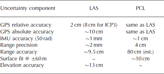
The LAS and the PCL share the same inertial measurement unit (IMU) system for position and orientation estimation. While the LAS is only able to obtain along-track measurements, our PCL scans over a swath (typically ∼200 m wide on the ground), from which it is possible to determine cross-track slope. Time-dependent scaling uncertainties in ranges produced by our PCL system (detailed below) require us to combine the PCL swath information with the stable range information provided by the LAS, for comparisons with the ICESat dataset. Both systems are mounted over a 45 cm diameter observation port in the underside of the aircraft, with the LAS mounted under the cabin floor and our PCL mounted in a rack over a hole in the cabin floor. During ICP4 and ICP5, the IMU was directly attached to our PCL’s body (Fig. 3); during ICP3 the IMU resided near the center of gravity (CG) of the aircraft.
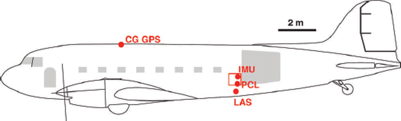
Fig. 3. Side-on view of survey aircraft, with installed locations of the center of gravity (CG) GPS antenna, IMU, PCL scan head and LAS.
Trajectory determination
GPS observations were recorded using an AeroAntenna AT1675-17 global navigation satellite systems (GNSS) antenna on the roof near the aircraft. Given the aircraft’s large ranges from GPS base stations (often >500 km), Precise Point Positioning (PPP) solutions independent of base stations were usually used, and solved both forward and backward in time. PPP solutions not coupled to the IMU had a typical uncertainty of 8 cm.
During the 2010/11 field season (ICP3), we used a real-time 50 Hz orientation solution from a Honeywell H-764 embedded GPS and inertial navigation system (EGI) loaned from the Danish Technical University (DTU), mounted in the center of the aircraft. Orientations were time-registered with position solutions from a 2 Hz Javad GNSS system acquiring data from the CG antenna. Due to occasional dropped data packets from the EGI, we were unable to perform loosely coupled merging of the EGI acceleration data and GNSS position data; however, accuracies consistent with altimetry were still obtained for most flights. The PPP positions were estimated for the CG antenna.
During the ICP4 and ICP5 seasons, we used a NovAtel OM-4 receiver recording at 1 Hz to obtain dual carrier phase data. An iMar FSAS IMU records raw acceleration and roll rate at 200 Hz. These data were processed after the field season using NovAtel’s Inertial Explorer package, with the ITRF 2008 reference system. Combined orientation/position data were output at 50 Hz estimated at the center of the FSAS unit, which was mounted 35 cm above the front of our PCL telescope. These combined position solutions were used as input for ‘loosely coupled’ position/orientation solutions, where the PPP data were allowed to control drifts on the IMU. In some cases with poor GPS observations a ‘tightly coupled’ solution was employed, where the orientation data were allowed to help triangulate the satellite range data.
Inertial Explorer’s estimate of the uncertainty for coupled solutions in vertical position is typically ∼2 cm; however, this estimate does not include systematic biases due to tropospheric delays, which may be several centimeters. Angular uncertainties are typically 50 rad.
Laser profiler
The LAS instrument has been used and validated in previous field campaigns (Reference Young, Kempf, Blankenship, Holt and MorseYoung and others, 2008a,Reference Young, Kempf, Blankenship, Holt and Morseb), and LAS data from ICECAP are available from the NSIDC (Reference Blankenship, Kempf and YoungBlankenship and others, 2012). The LAS is a Riegl LD90-3800-HiP-LR distance meter, with a 3.5 mW diode laser operating at 905 nm. The LAS acquires measurements at 2000 Hz, with a range resolution of 2 mm and ground spot width of ∼1 m. For each block of 575 pulses, the greatest range is recorded, along with the standard deviation and maximum amplitude of the detected pulse echoes. Typical point separation on the ground was 21–23 m, as expected for a target ground speed of 90 m s−1 . The maximum range of the system is 1500 m over ice.
To eliminate noise due to ground fog, clouds and regions of crevassing, we filter the range data to eliminate measurements with sample-to-sample jumps >2 m, and continuous runs of <20 samples. Short surface slopes of ∼5° or greater (rare on grounded ice on these lines) are filtered out. After the trajectory is obtained, for each time step we find the position and orientation in Earth Centered Earth Fixed space, and matrix translations are performed for the sensor lever arm and range vector, following Reference Vaughn, Bufton, Krabill and RabineVaughn and others (1996) and Reference KoksKoks (2008). The data are then transformed back to the WGS84 ellipsoidal reference frame.
Pointing bias determination
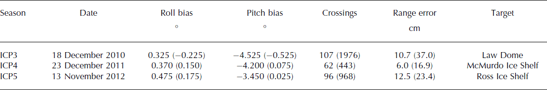
Geolocation of altimetry ranges requires accurate knowledge of the angular pointing bias between the source of orientation data and the laser vector. The milliradian precision needed for high-accuracy geolocation cannot be measured in a field installation, so typically these are determined from the altimetry data. The ATM group (Reference MartinMartin and others, 2012) uses repeated orthogonal passes over a stable flat surface, like an airport parking ramp. The LVIS group, using a high-altitude system, calibrate using roll-and-pitch maneuvers over flat, calm lakes or ocean (Reference HoftonHofton and others, 2000). Neither of these is readily available in Antarctica, with rapidly changing skiways or sea-ice infested coastal ocean being normal. We use elevation differences at orthogonal line crossovers to determine our pointing bias, and designed calibration flights to maximize crossovers of flat targets. We search the rollbias/pitch-bias space for the minimum root-mean-square (rms) crossover difference. Without accurate a priori data for the surface, range offsets are hard to determine, and can bleed into pitch-bias determination.
On Flight 23 of the ICP4 season, we conducted a gridded survey of the McMurdo Ice Shelf (Fig. 4). The line spacing was 2 km × 10 km over an area of 20 km × 100 km, yielding 100 line crossings. We edited out crossovers over crevassed ice; the results of the crossover minimization are detailed in Table 2. Similar calibration surveys were performed in ICP3 and ICP5.

Fig. 4. Surface elevation (curves, left scale) and derived crossover data (circles, right scale) used for laser pointing bias determination, acquired during ICP4/F23 over the McMurdo Ice Shelf on 23 December 2011. Background image is from MODIS (Moderate Resolution Imaging Spectroradiometer), acquired the same day (Reference Scambos, Bohlander and RaupScambos and others, 1996; updated current year).
Table 2. Results of ICECAP LAS crossover minimization (PCL values in parentheses)
Due to the bathymetric complexity of the McMurdo Sound, we did not correct for tides; based on GPS measurements on the ice shelf, we expect 8 cm rms difference between crossovers due to tides.
Laser profiler accuracy
For ICP4, we validate the accuracy of the LAS component of ALAMO against the 2003–09 ICESat record using data acquired on Flight 19 of the ICP4 season, in mid-December 2011. The target for this flight was a sparse grid south of Dome C, which is a region of low accumulation, low absolute accumulation variability and low slopes (Fig. 1, box c).
We obtain crossover differences between GLAH12.R33 data and Flight 19 LAS data, for points within 300 m of each other, and then bin the crossovers by operational period (Fig. 5). Using the LAS data as a benchmark, we find no evidence for a linear temporal trend in the Dome C ICESat elevation data. Over the whole ICESat interval, we find an ICESat crossover difference standard deviation of 9.5 cm on a 300 m baseline, a LAS–ICESat standard deviation of 13.1 cm, and a mean elevation bias of −12.5 cm for the LAS compared with ICESat. As the bias may be due to tropospheric effects on the GPS, we do not attempt to correct the entire record for this bias; instead, we use this term in our assessment of overall accuracy.
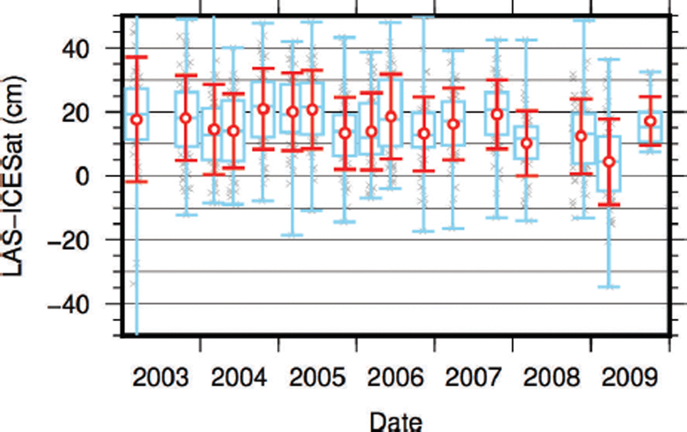
Fig. 5. Difference between ICESat and uncalibrated LAS elevations on ICP4/F19. Blue box-and-whisker plots show crossover quartiles and median for each epoch, while red shows standard deviations and means. Gray crosses are actual crossover differences. ICESat has a median offset of +12.5 cm from the LAS data; no temporal trend is visible.
Laser profiler elevation precision
We consider precision to be determined by the instrument’s crossover errors with its own data (equivalent to their relative accuracy), and accuracy to be determined by comparisons with other datasets. Note that in our usage, elevation precision includes an error contribution from any between-transect geolocation errors, while the running average approach is mostly sensitive to range measurement errors.
The ICP4 dataset contains 214 locations where two transects crossed within 3 days and adequate LAS data were recovered. Of these crossovers 49 were over grounded, uncrevassed ice. To determine the elevation precision of the LAS, we compare elevations of the closest georeferenced returns from different transects that are also within a 40 m radius on the surface.
Figure 6 shows a histogram of the differences in reported elevation for all crossings. The segments are ordered temporally, so any bias in Δz would indicate a change in elevation estimate correlated with time. If we assume that, for each crossing, both elevation estimates have the same variance and that their average is the true surface elevation, then for a single elevation measurement, we have
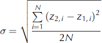
For non-crevassed grounded ice in the ICP4 season we estimate σ = 11.9 cm for LAS surface elevations.
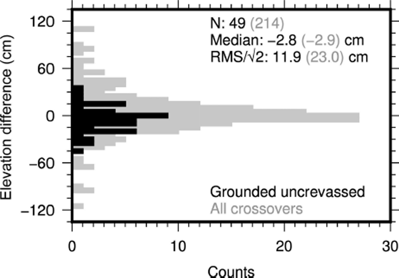
Fig. 6. Crossover difference histogram of ICP4 LAS data, binned at 5 cm intervals, with individual crossovers ordered by time and a maximum Δt of 3 days. No significant time trend is visible.
Photon-counting lidar
The concept of a PCL is described by Reference DegnanDegnan (2002). While the fundamental principles are similar to those of a traditional laser ranging system, a PCL relies on very fast pulse rates and statistical integration to allow detection of lower-energy returns, which results in substantial reductions in power, mass and optical structure requirements. These reductions enable the transmission of multiple discrete beamlets, with echoes received on individual counting cells, to cover both broad swaths of terrain and improved detection statistics. The scanning PCL system (Reference Degnan, Wells, Machan, Leventhal and BeckerDegnan and others, 2007; Reference HerzfeldHerzfeld and others, 2014) from which our PCL was derived was originally developed as an outer-planets exploration test bed, then adapted for deployment on unmanned airborne vehicles.
The ability to deploy a lightweight instrument with multiple lidar beamlets was a fundamental driver of the decision to use a photon-counting system, ATLAS, on ICESat-2 (Reference WuWu and others, 2010). Our PCL system differs from NASA’s Multiple Altimeter Beam Experimental Lidar (MABEL), a system specifically designed as an ATLAS simulator (Reference McGill, Markus, Scott and NeumannMcGill and others, 2013; Reference Brunt, Neumann, Walsh and MarkusBrunt and others, 2014), in that our PCL is typically flown at much lower heights (800 vs 20 000 m), has more counting cells (up to 100 vs 24) and actively scans vs. having fixed discrete beamlets.
Instrument description
In the ALAMO PCL a 532 nm, 19 kHz laser pulse is split into a 10 × 10 grid of beamlets and projected through a Risley prism beam steering unit (BSU), with time of the outgoing pulse recorded as the pulse ‘start’. The angular spread of the beamlets is 0.12°, yielding an illuminated grid on the ground of ∼1–2 m for every shot. For the ICP3 season, two prisms were used to generate a 45° linear scan pattern, with a maximum deflection from nadir of 14.9°. During the ICP4 and ICP5 seasons, only one prism was used, which resulted in a reduced circular scan pattern with 7.3° deflection from nadir (Fig. 7). The BSU is synchronized to the laser, such that one cycle of the BSU corresponds to 1024 shots after the system has ‘spun up’ after starting; thus the system scans underlying terrain at 18.5 Hz.

Fig. 7. Scan pattern for ALAMO during the ICP4 and ICP5 seasons, showing coverage over 1 s, assuming a height above ice of 800 m and an aircraft velocity of 90 m s−1 to the right. The final complete PCL scan is shown in green. Subset ‘pseudobeams’ are numbered 0, …, 5. The LAS footprint is shown in red. The nadir point for the final scan is shown by the cross.
Return photons are received through the same optics and directed to a 10 × 10 counting cell anode micro-channel plate photomultiplier. Timing of the returns is split 50/50 between two independent field-programmable gate arrays (FPGAs). Each counting cell has a coarse, 16 bit ∼295 Hz clock (range resolution ∼0.5 m) and a fine 8 bit ∼12.5 GHz clock (range resolution ∼1.2 cm), calibrated per shot that allows ∼0.1 ns precision for detection times (‘stops’). The differences between the starts and stops is the time-of-flight, which when multiplied by an appropriate velocity of light provides the apparent range to the photon source. A range gate is applied to limit incoming photons on our PCL; this is adjusted to match the aircraft’s height above ice, and was typically 1000 m tall, centered at a distance of 1000 m.
An important constraint on the use of this dataset relates to the stability of the coarse clock. The coarse clock rate can drift, due to temperature and hardware issues, by up to 0.01%, limiting absolute range accuracy to 80 cm without registration to the LAS.
The 0.7 ns pulse width limits the precision of start times, yielding a minimum range precision per photon of ∼10.5 cm. Systematic biases between individual counting cells are symmetrically distributed with a rms deviation of 15 cm. We calibrate these biases within the resolution afforded by the pulse width. Higher precision requires stacking numerous individual shots and channels.
Time stamps are generated with every shot, every prism rotation and on reception of a 1 Hz GPS generated pulse for timing calibration. The timing data from each FPGA is recorded directly to independent hard drives, typically at 4–5 MB s−1 . In post-processing, these time stamps allow each photon’s time-of-flight to be converted into an X, Y and Z location relative to the sensor.
PCL surface detection and geolocation
There are two key challenges when working with data from a scanning PCL. First, properly georeferencing photons from up to 14° off nadir requires knowing the aircraft’s orientation and the sensor’s relative pointing biases with milliradian accuracy. Second, a PCL produces large volumes of data with a low signal-to-noise ratio. This demands computationally efficient approaches that use statistical inferences to determine the true surface within a spatial volume contaminated by solar photons (Fig. 8) and superposed electronic noise (Fig. 9). Our approach to addressing this challenge in post-processing involves subsampling the photons into ‘pseudo-beams’, chosen to mimic the planned ATLAS configuration, detecting a surface while still in the aircraft-relative frame, and finally georeferencing that surface point. This product both minimized the amount of data required to determine the pointing biases, and for estimating cross-track slopes.
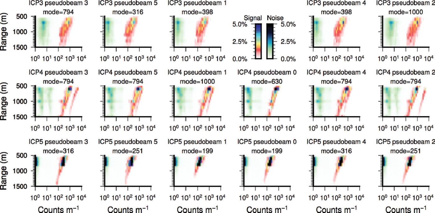
Fig. 8. Distribution of signal (right of plots) and noise (left of plots) photons used for the ALAMO analysis as a function of range and intensity for each season and pseudobeam. Counts are detections per 5 m range interval, per 0.25 s integration interval. Plots are positioned according to their location within the scan pattern; there is no pseudobeam 0 for ICP3. Noise values are the average counts in a 50 m range interval 75 m ‘above’ the surface return. For typical flight heights, signal-to-noise ratios are approximately two orders of magnitude, dropping to one order of magnitude at the far edge of the range gate. Lower signal intensities in ICP5 are matched with correspondingly lower noise values, suggesting variations in the detector gain.
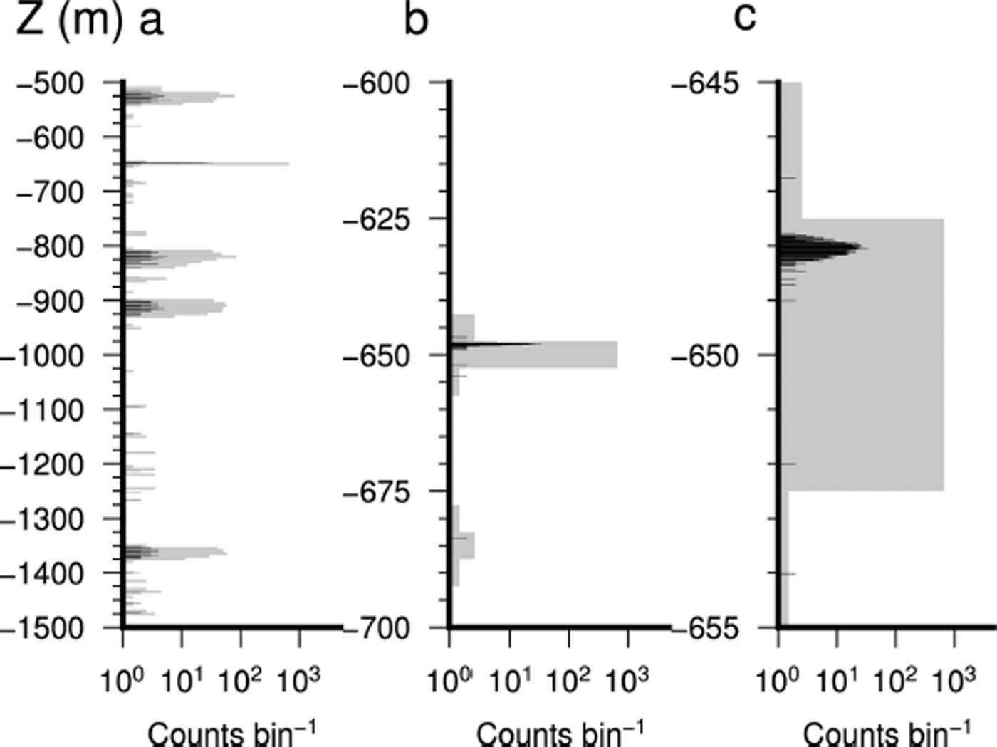
Fig. 9. Three views of a single Z range histogram for beam 0, from ICP4 Flight 13. Gray bars show the coarse 5 m histogram, and black bars show the fine 1 cm histogram. Note the logarithmic scale. (a) The full range gate; the sharp peak at 649 m is the surface, and broader peaks are electronic noise. (b) Zoom-in on the coarse peak. (c) Detail of the fine peak – the median of this distribution is chosen as the surface.
Data subsetting
The objective of pseudobeam averaging is to generate a simple data product of manageable volume that can be used both to iteratively determine pointing biases and to accomplish first-order altimetry science goals. To do this we emulate the discrete beams found on the ATLAS system by filtering for photons within limited cones. For circular scan patterns, we selected six cones within the lidar reference frame (Fig. 7), sampling the edges, fore and aft, and at 45°. For linear scan patterns, we selected the edges of the scan pattern, the nadir point and two points in between. The typical cross-track spacing between the along-track and mid-cross-track pseudobeams is 70–100 m, similar to the 90 m separation of the planned ATLAS beams. Each pseudobeam consists of the photons within a single cone over 0.25 s (∼5 scans). At typical aircraft survey heights, this cone corresponds to a 10 m × 25 m footprint for each pseudobeam. For each pseudobeam, a range to the surface is computed and the resulting vector is georeferenced. This approach greatly reduces the data volume, while preserving information content about the extrema of the scan pattern. A version (Reference Blankenship, Kempf, Young and LindzeyBlankenship and others, 2013b) of this dataset (with geolocated photons) is available from NSIDC.
Surface detection
To determine the surface location, we extract ranges from the pseudobeam’s subset photon cloud. For each pseudobeam, we first build a histogram along the Z vector of our PCL coordinate system with 5 m (coarse) bin resolution (Fig. 9). The maximum bin is selected as the coarse Z distance. The average of a 10 m window centered on 15 m is used to assess solar photon levels. Points where the peak coarse bin count is <50, or the coarse signal-to-noise ratio (SNR) is <2.5 are excluded from the subsequent analysis. To determine a more precise location, we return the median Z distance of photons in the maximum coarse bin and the two adjacent bins. Given typical SNRs of 100 (Fig. 8), we estimate the precision of the 40 cm wide integrated pulse to be
Using the known angles for this pseudobeam and the computed distance to the surface in the Z-direction, we calculate X-distance and Y-distance in our PCL’s reference frame. We then geolocate the surface range vector using the method used for the LAS system. Photon counts for the peak coarse and fine bins, the background noise rate, and information on the shape of the integrated surface return are also reported. These data are distributed by NSIDC as part of Operation IceBridge’s ILSNP4 data (Reference Blankenship, Kempf, Young and LindzeyBlankenship and others, 2013a). Locations of ILSNP4 PCL surface elevation data in the Wilkes Land region of East Antarctica are shown in Figure 1.
Surface-Elevation Change Determination
For this paper, we use the ILSNP4 slope and elevation data product to assess the linear, invariant component of surface-elevation change over the ICESat record, as constrained by the ALAMO cross-track slope product. We also use the ILSNP4 data to investigate the surface-elevation change since the end of the ICESat record, for which ICECAP represents a unique record.
Slope derivation
We derived surface slope using geolocated PCL beam surface detections within 200 m of each LAS point to determine a best-fit plane specified by
where a, b and c are constants defining the slope, x and y are eastings and northings in the standard polar stereo-graphic projection, and z is elevation in the WGS84 coordinate system. z at the location of the LAS coordinate is fixed to the LAS elevation. Solutions that are not constrained by at least ten points from a side-pointing pseudobeam are rejected, as are solutions where the centroid of the PCL points is >66 m from the LAS spot. We used a linear least-squares method to perform the fit, and output the standard deviation of the residuals, as well as the slope parameters.
These combined surface-elevation and slope estimates are included in the ILSNP4 Hierarchical Data Format 5 (HDF5) data product available from NSIDC (Reference Blankenship, Kempf, Young and LindzeyBlankenship and others, 2013a).
Linear ALAMO–ICESat dz/dt determination
Using the ALAMO slope parameters, we find all ICESat foot-prints within 200 m of each LAS spot measurement. We use
to estimate the ALAMO elevation at each ICESat point, and find the elevation differences, ΔzI−A, and the time separation Δt I−A, where ‘I’ and ‘A’ indicate ICESat and ALAMO, respectively. We filter out ICESat footprints with Δz I−A > 20 m, interpreting them as non-physical. For each LAS spot, we solve
as a linear fit to these two vectors, requiring a minimum of four ICESat footprints. dz/dt is the time-invariant rate of surface-elevation change, and C is the difference between expected and observed elevations if this trend had continued to the time of the ALAMO observation. From the residuals we estimate the R 2 of the fit and combine the residuals with the number of footprints to find the 95% confidence intervals assuming a χ 2 distribution. For this analysis, no binning or filtering of the trends obtained is performed beyond this step to further elucidate the sources of uncertainty.
Post-ICESat elevation change
C should be equal to zero if linear trends identified above continue to the time of the ICECAP observation. If the 2003–09 dz/dt trend is significant but C is larger than the instrument errors, this would imply a change in behavior of the system. Where the ICESat era trend is significant, we convert C into the linear rate required to match the end of the ICESat time series to the ALAMO observation using the equation
where dz/dt is elevation rate of change over the ICESat period and dt ICESat is the time between the end of the ICESat time series and the ALAMO observation. Propagating the 13 cm elevation error we estimate for LAS elevations (the ultimate source of ALAMO surface elevations) through this equation leads to an uncertainty of 7 cm in ICP3 and 3.5 cm in ICP5 due to ALAMO. The bulk of the uncertainty is in the trend-line estimate of C. We therefore restrict this analysis to ICESat era trends with an R 2 value of at least 0.8.
Results and Analysis
Wilkes Land overview
Wilkes Land and the adjacent George V Land of the Indo-Pacific sector of the Southern Ocean adjoins a region of the East Antarctic ice sheet underlain by deep subglacial basins that bear evidence of considerable past retreat (Reference Jordan, Ferraccioli, Corr, Graham, Armadillo and BozzoJordan and others, 2010; Reference YoungYoung and others, 2011) and current sub-glacial activity (Reference Smith, Fricker, Joughin and TulaczykSmith and others, 2009; Reference WrightWright and others, 2012; Reference McMillan, Corr, Shepherd, Ridout, Laxon and CullenMcMillan and others, 2013). As these basins are grounded below sea level and slope toward the interior, the overlying ice sheet is susceptible to rapid retreat through the marine ice-sheet instability if restraining forces on the sides and front are released, in particular from bounding ice shelves (Reference SchoofSchoof, 2007).
Estimates from ice divergence indicate that basal melt rates are currently low at Cook Ice Shelf (Reference Rignot, Jacobs, Mouginot and ScheuchlRignot and others, 2013), and evidence of current ice loss from the grounded ice inland from spaceborne repeat altimetry (Reference Pritchard, Arthern, Vaughan and EdwardsPritchard and others, 2009) and gravity (Reference Chen, Wilson, Blankenship and TapleyChen and others, 2009; Reference Luthcke, Sabaka, Loomis, Arendt, McCarthy and CampLuthcke and others, 2013) has been ambiguous.
Totten Glacier is one of the largest glaciers on Earth and has exhibited consistent lowering across the satellite record (Reference Davis, Li, McConnell, Frey and HannaDavis and others, 2005; Reference ZwallyZwally and others, 2005; Reference Flament and RémyFlament and Rémy, 2012; Reference Khazendar, Schodlok, Fenty, Ligtenberg, Rignot and Van den BroekeKhazendar and others, 2013), although rough terrain and pervasive cloud cover make it a difficult target for radar and optical systems, respectively.
Denman Glacier represents another outlet of the Aurora Subglacial |Basin, and from satellite data has also exhibited lowering trends, associated with a dynamical ice shelf. However, due to its location in a pronounced valley in the ice sheet, and association with exposed nunataks and blue-ice regions, it has been hypothesized that the lowering may be due to enhanced wind erosion (Reference Flament and RémyFlament and Rémy, 2012).
Results at Cook Ice Shelf
As part of the ICECAP project, three ICESat reference tracks (0277, 0001 and 0039) in this region were targeted for overflight by ALAMO on Flight 13 of the ICP4 field season. This area is prone to significant cloud interruptions; the top panel of Figure 10 shows the number of successful repeat tracks dropped to six near the grounding line on ICESat track 0001, impacting the stability of ICESat-only fits (as can be seen in the expansion of the pink confidence intervals). Residuals for the ALAMO fit remain low (30 cm) on track 0001, implying that a planar fit is appropriate for the region surveyed, despite significant surface slopes. The confidence intervals provided by ALAMO (in blue) provide compelling evidence that any regional linear trend in surface elevation must be under ±30 cm a−1, and is indistinguishable from zero. The derived rate from C (not shown for clarity) is within the confidence interval of the ICESat era rate.
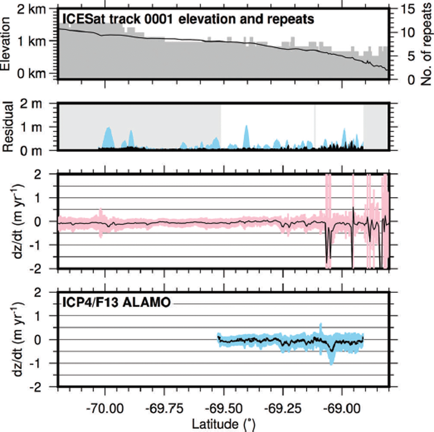
Fig. 10. Elevation change over a Cook Ice Shelf tributary. ALAMO data were collected on 3 December 2011 during ICP4. Top panel shows the ICESat-derived ice-sheet profile, and the number of successful ICESat repeats between 2003 and 2009. Second panel shows the residuals to the ALAMO fit (black), the expected residuals due to uncorrected cross-track slope (based on the slopes derived from ALAMO, blue); white background shows where the aircraft track was within 100 m of the ICESat reference track. The third panel shows ICESat-derived dz/dt with a 95% confidence interval (pink). The bottom panel shows ALAMO-corrected ICESat dz/dt with a 95% confidence interval (blue).
The result of little change in surface elevation is consistent with observations of limited melt rates inferred below Cook Ice Shelf (Reference Rignot, Jacobs, Mouginot and ScheuchlRignot and others, 2013), and thus reduced sensitivity to ocean variability. Gravity Recovery and Climate Experiment (GRACE) observations do indicate mass loss in this region (Reference Chen, Wilson, Blankenship and TapleyChen and others, 2009); however, due to the low resolution of spaceborne gravimetry, mass loss may be due to an adjacent catchment.
Results from Wilkes Land
Our dz/dt analysis was extended to the two key glaciers further west in Wilkes Land, using data from the ICP3 and ICP5 seasons, where we find evidence for much more rapid change than at Cook Ice Shelf.
The most prominent changes over the ICESat–ALAMO observation period are found over Denman and Totten Glaciers, along tracks 1335 (Fig. 11) and 0033 (Fig. 12), respectively. Each of these tracks was repeated in the ICP3 and ICP5 seasons. We find maximum rates of surface lowering for the ICESat epoch of −1 m a−1 on a fast-flowing interior bend of Denman Glacier, and −2 ma−1 near the grounding line of Totten Glacier (also identified by Reference Khazendar, Schodlok, Fenty, Ligtenberg, Rignot and Van den BroekeKhazendar and others, 2013).
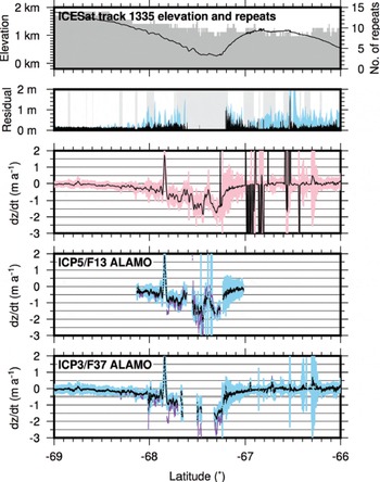
Fig. 11. Elevation change over Totten Glacier, which lies between Law Dome (latitude −67 to −66°) and the bulk of the East Antarctic ice sheet. ALAMO data were collected on 30 December 2010 in ICP3 and 1 December 2012 during ICP5. Key is the same as Figure 10; the fifth panel shows ICP3 ALAMO data. The purple line represents the post-ICESat dz/dt trend required by C; we only estimate this trend where the ICESat interval trend has R 2 > 0.8.
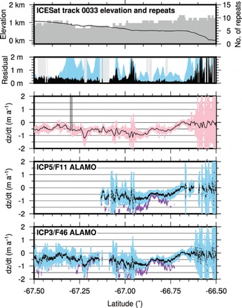
Fig. 12. Elevation change over the edge of Denman Glacier, between the Obruchev Hills (−66.6° to −66.5°) and the shear margin of Denman Glacier (south of −67°). ALAMO data were collected on 18 January 2011 during ICP3 and 30 November 2012 during ICP5. Key is the same as Figure 10; the bottom panel shows ICP3 ALAMO data.
Totten Glacier
In both the ICESat-only case (pink in Fig. 11 third panel) and the ALAMO-corrected datasets the hypothesis of no linear trend can be rejected, with confidence intervals of ±25 cm for most of the region. One region where the planar assumption used for both ICESat-only and ALAMO datasets appears to degrade is the south side and summit of Law Dome. This region of Law Dome is dominated by blue ice and steep ice slopes; increased residuals (and a corresponding increase in the size of the confidence interval) are apparent.
For Totten Glacier, we find in general that the difference in ICESat and post-ICESat trends is within the 95% confidence interval, implying no significant changes in lowering. An exception is linked to a 5 km wide prominent spike of surface-elevation growth during the ICESat era at −67.8°, focused on a downstream stepping 200 m bed relief feature. This feature may represent a localized subglacial hydraulic feature with time-varying behavior, and is linked to the interior subglacial hydrological network (Reference WrightWright and others, 2012).
Denman Glacier
Track 0033 (Fig. 12) samples a variety of different terrains in Wilkes Land, including the Obruchev Hills, a complex of nunataks and blue ice on the ice-sheet slope, marginal ice feeding the main trunk of Denman Glacier (between −66.6 and −66.95°), and the shear margin of Denman Glacier. It is also in a cloudy portion of the Antarctic coast, with <10 repeats available for ICESat analysis. We find (as expected) very high residuals over the Obruchev Hills, and also while crossing the shear margin of Denman Glacier. We find in the marginal ice a progressive increasing lowering rate from −50 cm a−1 to −1 m a−1 as the shear margin is approached. When examining the implied post-ICESat rates (purple curves in Fig. 12), we find that rates over the shear margin of the glacier appear to have doubled. These observations would be consistent with a slowing of the main glacier trunk, followed by a kinematic wave propagating upstream.
Conclusions
During the course of NASA’s Operation IceBridge, ICECAP collected 25 039 track kilometers of re-flights of ICESat lines over the margins of the East Antarctic ice sheet. The Airborne Laser Altimeter with Mapping Optics (ALAMO), a scanning photon-counting lidar registered to a nadir laser profiler, was deployed to extend the elevation record of ICESat. We find the ALAMO dataset meets IceBridge science requirements and can confirm and enhance the ICESat record in Antarctica.
With our record along existing ICESat lines we find little evidence of broad surface-elevation change in the region feeding Cook Ice Shelf, indicating a relatively stable system there. Conversely, our observations show continued dramatic ice lowering at Denman and Totten Glaciers, likely driven by changes in the floating portions of the glaciers caused by enhanced ice-shelf melting. We also find evidence of localized surface-elevation change, consistent with subglacial hydrology. This paper represents the first demonstration of swath photon-counting altimetry over Antarctica and sets a precedent for ATLAS observations over ice sheets following the launch of ICESat-2.
Acknowledgements
Funding for the fieldwork and data reduction was provided by NASA grants NNX09AR52G, NNG10HP06C and NNX11AD33G, Program DACOTA (06-VULN-016) of the Agence Nationale pour la Recherche, and UK Natural Environment Research Council grant NE/D003733/1. This work was supported by the Australian Government’s Cooperative Research Centres Programme through the Antarctic Climate and Ecosystems Cooperative Research Centre (ACE CRC). This work received funding from the American Recovery and Reinvestment Act. Logistical support was provided by Australian Antarctic Division (through Australian Antarctic Programme projects 3103 and 4077), the US Antarctic Program and the French Polar Institute. We thank DTU for their loan of an EGI and thank Gabriel Jodor and Christopher Field of Simga Space Corporation for technical guidance with this system. We thank Chad Greene for reviewing drafts of this paper, and Tom Neumann, an anonymous reviewer and the scientific editor, Helen Fricker, for valuable suggestions. This paper is UTIG contribution No. 2699.


