Setting down the problem
Rationale of modelling
Let us begin with rather philosophical considerations. Glacier dynamics, the application of the laws of mechanics and physics to glacier flow, is only possible after a composite model has been submitted for the real situation. Models must be chosen for the geometry of the glacier and its bedrock, for the rheology of ice, for the balances at the surface, for the water circulation, etc. The best model is that which fits the largest number of observations with the least complexity. While doing this three points must be kept in mind:
-
1. A model is a simplification of reality which has been constructed with some goal in view. It must not be used for another purpose without reconsidering again the actual situation. For instance, in order to calculate the stresses, a bedrock may be replaced by a perfectly smooth surface, ignoring any scratch or rock joint. We cannot deduce from this model that the ice-bedrock surface is perfectly watertight.
-
2. A realistic model should lead to the phenomenon or to the numerical value which is actually observed, but the converse is not true. The reproduction of a phenomenon (e.g. periodic surges) or obtaining a plausible numerical value (e.g. a correct sliding velocity) is not proof that the model is realistic. Intermediate values and processes must be checked too, not only the final result.
-
3. Once a model has been constructed, even if it is a very rough one, it must be handled with rigour. Rigour does not mean exact analytical solutions; it means only that approximations are clearly stated as such. But in glacier sliding theory several analytical solutions have been guessed without the beginnings of a proof.
In this article we shall give a didactic account of the friction laws trying not to fall into any of the pitfalls mentioned.
Definition of the sliding velocity
To tackle glacier dynamics, the first model to be adopted is the shape of the glacier (or ice sheet). Its actual shape must be sufficiently smoothed to be represented by an analytical or a simple geometrical surface, thus allowing calculations.
The boundary conditions for this smoothed glacier are: no stresses on the upper surface, and some relation giving the shear stress on the smoothed bedrock τb as a function of the sliding velocity U. This relation, which will be called the friction law, is assumed to vary in a continuous, smooth way from place to place. Then the flow solution for the smoothed glacier may be assumed also to be smooth (instabilities producing narrow shear zones, faults, and cracks are assumed not to exist).
To match the real glacier, the bottom shear stress in the smoothed model must be the average of the real shear stress on the same geometrical surface. When the real stresses are replaced by smoothed values, the equilibrium conditions still hold.
For the velocities it is not the same, because the ice is not Newtonian viscous. The real stresses produce fluctuating strain-rates near the bottom, according to the ice creep law. This ice creep law does not hold between the average stresses and the average velocities. Thus the average real sliding velocity at the bottom, say Ū, differs from U. Since the stress fluctuations at the bottom in the real glacier lower the viscosity, Ū > U.
The z-axis being perpendicular to the smoothed bedrock, let ū(z) be the locally averaged real forward velocity, which becomes Ū on the smoothed bedrock, and u(z) the forward velocity in the smoothed problem, which becomes U at the bottom. In the case of a wavy bedrock with very small slopes (relative to the smoothed bedrock) it has been shown (Reference LliboutryLliboutry, 1975) that Ū—U≪U, but that ∂(ū—u)/∂z is not at all negligible. Thus, although the additional sliding Ū—U (already introduced by Reference KambKamb, 1970) may be neglected, the tilt-rate of bore holes near the bedrock cannot be analysed as this author did, in order to obtain an appropriate value of the exponent n in Glen’s law.
The friction law
Glacier dynamics has then been split into two problems.
Problem I: the dynamics of a smoothed glacier, having a basal shear stress (the glacier friction) τb and a sliding velocity U.
Problem II: the friction law, which should give τb as a function of U and of other local variables. This friction law may be determined, at least theoretically, from consideration of the processes at the bottom of the glacier.
Solving the first problem will give τb as a function of the geometry of the smoothed glacier and (perhaps) of the body velocities. For instance, in the two-dimensional case (with z-axis upwards, and x-axis forward), when the body stresses, the surface slope (α > 0), the thickness h, and the vertical velocity at the surface are all independent of x (a situation called Nye flow, Reference LliboutryLliboutry, 1964–65, Tom. 2, 1971).

where ρg is the specific weight of ice.
The analysis of a kinematic wave studied by J. Vallot (Reference LliboutryLliboutry, 1958, 1964–65, Tom. 2, p. 638–40) lead us to the conclusion that Equation (1) fails for a valley glacier: τb depends on the thickness, slopes, and bends of the valley over a long distance (see also Reference Bindschadler, Bindschadler, Harrison, Raymond and CrossonBindschadler and others, 1977). Reference Shumskiy, Nye and ShumskiyShumskiy (1965) arrived at the same conclusion from the existence of reverse superficial slopes in ice sheets over large distances. As a matter of fact for a smoothed ice-sheet with small surface and bottom slopes, in the two-dimensional case, τb is given by the relation (Reference BuddBudd, 1968)

where b(x) is the bottom smoothed profile, b(x)+h(x) the smoothed surface profile, and ![]() the longitudinal deviatoric normal stress. It is only when averaging Equation (2) over very long distances, at least 20 times the glacier thickness, that Equation (1) may be obtained.
the longitudinal deviatoric normal stress. It is only when averaging Equation (2) over very long distances, at least 20 times the glacier thickness, that Equation (1) may be obtained.
Solving the second problem will give τb as a function of the microrelief of the bedrock, the characteristics of the bottom ice–debris layer (a moving basal moraine) or the subglacial loose drift when they exist, the sliding velocity U, the average normal pressure of ice against the bed p∞ , the pressure p of subglacial water (in the interconnected regime, to be defined later) or its total amount per unit area (in the autonomous regime, to be defined later), etc. Weertman has said that our approximate law for fast-sliding glaciers, namely:
is incomplete because p is unknown. However, it is not the friction law which is incomplete, it is the modelling of glaciers. If p appears to be a crucial variable in the friction law, then a model of glacial hydrology which can lead to realistic values of p must be constructed. This is a third problem of glacier dynamics, needing to be studied and solved separately.
In order to model glacier surges, Reference BuddBudd (1975) introduces a so-called “friction law”, which for a very large ice sheet (s = 1 in Budd’s paper) may be written:

where ![]() is an x-independent but time-dependent parameter, Φ a constant, V the average velocity from surface to bottom. Equation (4) is not a friction law. In particular, since in Budd’s theory ρghα differs significantly from τb
, it cannot enter into a friction law. Equation (4) is an equation expressing arbitrary feed-back between τb
and V which is substituted for both the lower boundary condition and the hydrological model. The fact that this feed-back produces periodic surges, and that Φ may be chosen in order to match the actual periodicity of surging glaciers is no proof of its validity, as stated before.
is an x-independent but time-dependent parameter, Φ a constant, V the average velocity from surface to bottom. Equation (4) is not a friction law. In particular, since in Budd’s theory ρghα differs significantly from τb
, it cannot enter into a friction law. Equation (4) is an equation expressing arbitrary feed-back between τb
and V which is substituted for both the lower boundary condition and the hydrological model. The fact that this feed-back produces periodic surges, and that Φ may be chosen in order to match the actual periodicity of surging glaciers is no proof of its validity, as stated before.
Glacier dynamics at different scales
Only ice sheets resting on a bedrock without any continuous and more or less mobile layer of drift at the interface will be considered in this article. Let us come back to the problem of smoothing the glacier shape, or, in other words, of determining which irregularities must be considered as the roughness, the microrelief of the bedrock, and which ones as the general shape of the glacier.
Three kinds of irregularities may be found:
1. Protruding obstacles, with a width of the same order of magnitude as their height. They will be called knobs, whatever may be their size. (Hollows of the same kind may be neglected, since in general they are infilled with drift.) For these knobs we must choose a cut-off size R M.
2. Transverse undulations, with a width one order of magnitude larger than their height, which will be called bumps. The flow over a bump is more or less two-dimensional, and thus only the longitudinal profile of the bedrock is significant. As explained by Reference NyeNye (1969) we must then choose an averaging length A to smooth the profile. More precisely, we may first substitute for the actual profile at very large distances (larger than the length of the glacier if necessary) a curve tending very swiftly to a straight line (z = 0), in order to be able to define the Fourier transform of the profile b(x), say:

where ν = 1/λ is the wave number. Next we may split the full Fourier spectrum by some cut-off wave number ±1/A. According to the fundamental relation of convolution:

the corresponding averaging function f(X) is:

3. Channels approximately in the direction of flow, with a fluctuating width, or undulating between left and right. For a valley glacier, the valley itself may wind. To take this into account, a two-dimensional Fourier transform is needed. For sake of simplicity we shall not consider this case.
In this article only local friction laws will be considered. The height of the biggest knobs or bumps of the microrelief over the smoothed bedrock is assumed to be an order of magnitude smaller than the glacier thickness. For this, in general, a cut-off wavelength A as large as the glacier thickness may be assumed, but a still smaller value (of the order of 30 m for an Alpine glacier) is necessary for the following reason. In the “interconnected subglacial hydraulic regime” we shall consider interconnected water bodies at the ice-bedrock interface, with a negligible head loss between. In order to have more or less the same pressure p in all these cavities, they must be more or less at the same altitude.
Starting from the local friction law, for a valley glacier, a first step will be to average the friction over all the cross-section of the glacier. The interconnected cavities, in our model, will be connected with a main waterway at altitude Zw , where the pressure is p w. Then with ρwg denoting the specific weight of water and Z b being the altitude of a cavity with pressure p,
The local friction law, Equation (3), and this relation, Equation (8), have been used by Reference ReynaudReynaud (1973).
A further step, not dealt with in this article, will be to average the friction over a long distance, taking into account the variation of p
w (in the steady state, Röthlisberger’s theory (1972) may be used). For the body of the glacier τ
b must be averaged over this long distance and as said formerly in many cases, 〈〉 denoting the averages, we may write 〈τ
b〉 = ρg 〈h sin α〉. This is not the case for a small glacier, where in Equation (2) the last term on the right side is negligible and ![]() decreases in the direction of flow from the bergschrund to the front. It is also not the case for a winding valley glacier. Thus the way from the local friction law to the global dynamics of a glacier, to the scale at which kinematic waves or surges must be studied, is not so simple as commonly thought.
decreases in the direction of flow from the bergschrund to the front. It is also not the case for a winding valley glacier. Thus the way from the local friction law to the global dynamics of a glacier, to the scale at which kinematic waves or surges must be studied, is not so simple as commonly thought.
Assumed models
A model for ice rheological law
In temperate glaciers, the peculiar ice fabric with the optical axes clustered in several (generally four) maxima is found to the very bottom. Reference DuvalDuval’s (1977[a], in press) studies have shown that the creep of ice with this peculiar ice fabric involves:
-
(1) A reversible creep, logarithmic at first and coming to a stop (at constant stress) after less than one hour. The final strain is proportional to the stress, almost insensitive to temperature, and one order of magnitude larger than the standard elasticity which is relevant for sonic or ultrasonic waves. Phenomenologically it is a delayed elasticity (Duval’s pseudo-elasticity). Duval explains it by a reversible motion of tilt boundaries between sub-grains.
-
(2) Andrade’s transient creep, which is proportional to the one-third power of the time and to the cube of the stress, strongly temperature-dependent, and irreversible.
-
(3) A tertiary permanent creep, sometimes at a fluctuating rate because strain-hardening and recovery prevail in turn. On the average it follows Glen’s law with n = 3 in the range of stresses which is found in the body of glaciers. (Experiments for higher stresses such as are found in the vicinity of a knob are in progress).
According to Duval, when the deviatoric stresses τ ij′ change by Δτ ij′ at time t = 0, the total strains after less than one hour are modified by
where τ is the effective stress defined by

In the following Duval’s pseudo-elasticity, Andrade’s transient creep, and the fluctuations of the tertiary creep rate will be ignored, although for fast sliding velocities they are not negligible. In particular pseudo-elasticity (and perhaps also a fluctuating creep-rate) could explain the jerky sliding observed by Reference Vivian and BocquetVivian and Bocquet (1972) in a large cavity under Glacier d’Argentière. There the glacier slides suddenly by about 2 cm at instants several hours apart. To explain this phenomenon by a stick-slip movement, a Young modulus of the order of 105 N would be necessary. The elastic Young modulus of ice is 9.2 × 10⁵ N, but Duval’s “pseudo-elastic” modulus is the correct value.
In general the sliding velocities are of the order of 10 cm per day or less. Since (as we shall see) the bumps which afford most of the friction have a length between 10 cm and 1 m, Andrade’s transient creep should not modify the friction over bumps very much. Nevertheless when sliding over knobs occurs, it could.
Another fact is the variability of the parameter B at the melting point according to grain size, salt content, and, above all, liquid-water content (Reference DuvalDuval, 1977[b]). The heat dissipation within the bottom ice should continuously increase its water content. Since this is obviously not the case (at the snout the liquid-water content of bottom ice remains low), active ice cannot be perfectly impervious, but must allow water to exude to the ice–bedrock interface. This is consistent with the fact that, from the analysis of the air entrapped in the bubbles, Reference Berner, Berner, Stauifer and OeschgerBerner and others (1978) have estimated the amount of water which migrates downwards through Gornergletscher to be about 4 cm per year. Thus an equilibrium between water production and its exudation should be obtained after a short length. A periodic variation between the up-slopc and down-slope sides of an obstacle should remain; it will not be taken into account.
This drainage should purify bottom ice, and we may neglect its salinity Reference Lliboutry(Lliboutry, 1976). Finally, in active bottom ice, grain size also should reach a steady value. Thus B may be considered as a constant for the bottom ice of all active temperate glaciers.
To summarize, the model for bottom ice will be a Glen body that is a material with the following rheological law:
where B and n are constants. For n = 1 (a Newtonian viscous ice), and no ice–bedrock separation, since all the equations and boundary conditions are linear, τ b should be proportional to the sliding velocity U. For B =τ c −n and n → ∞ (a perfectly plastic ice), without ice–bedrock separation, τ b = τ c, but if τ c ≫ τ b, there is extensive ice–bedrock separation and it is well known that the solid friction law Equation (3) becomes roughly valid.
Energy balance in the meltitig–refreezing process
By saying that “there is no ice–bedrock separation”, we mean that there only exists between ice and rock a water film of micrometric thickness. This water film is a consequence of the melting–refreezing process which allows ice to slide over minute obstacles. Reference NyeNye (1973) has calculated its thickness in the case of a microrelief with a sine profile, assuming the slopes to be small and the ice to be Newtonian viscous. He has shown that a water film of the order of 1 mm, with water flowing in the direction of glacier flow everywhere, as assumed by Reference WeertmanWeertman (1972), would be unstable. We shall here complete Nye’s calculation by showing how the Newtonian energy lost by the corresponding sliding at velocity U f, that is U fτ b , per unit area and time, turns into heat.
Let us consider a bedrock profile
and ice with a Newtonian viscosity η. The normal pressure on the bedrock for a total sliding velocity U is found to be Reference Lliboutry(Lliboutry, 1975)
whence a drag
where

The constant ω*, to which corresponds the controlling wavelength λ*, will be defined later. We may write
U p and U f being the slidings by plasticity and by melting–refreezing respectively. The ice velocity in the upward direction at the ice–bedrock interface is found to be,
whence a melting-rate per unit width,

ρ and ρ w denoting the density of ice and water respectively.
Now the discharge per unit width of a water film of thickness t is

η w being the viscosity of water. Whence, comparing Equations (18) and (19), Nye’s value of t is found by solving

The heat dissipation within the water film, due to the viscosity of water, is — q(dp n/dx), and, on average:

according to Equation (14), (15), and (16). Thus 90% of the Newtonian energy which is lost appears as heat in the water film.
To account for the missing 10% consider 1 g of ice which melts at pressure p n (given by Equation (13)) and temperature T = T∞ — Cp n, absorbing latent heat L. This gramme of water with a heat capacity c w warms from T to T’, where it refreezes at pressure pn ′ giving latent heat L′. Next this ice, with a heat capacity c i cools from T′ to T, where it melts again, and so on. Melting and refreezing took place along the same flow line, which is partially in ice, partially in the water film (Fig. 1), and thus the process is strictly periodic. The total production of heat during a cycle per gramme of ice is then —L—c w(T′ — T) +L′ + c i (T′ — T). Now, from classical thermodynamics:


Thus the heat production per cycle and gramme of ice is:

In the interval (x, x + dx), per unit width and time, according to Equation (18), it freezes ρ U(a—ap) ω sin ωx dx grammes of ice. This ice melts for an opposite value of sin ωx, and then in Equation (24), according to Equation (13),
The heat production per unit area and time is

according to Equations (14) and (16).

Fig. 1. Flow lines in the regelation ice and in the water film of micrometric thickness. In the melting—refreezing process of sliding, the heat balance of the periodic changes of state, of the cooling of the ice and the warming of the water, amounts to 10% of the Newtonian energy which is lost. The main part is lost by viscous dissipation in the water film.
A model for subglacial water
The total frictional heat, Uτ b per unit area and time, which is dissipated in the sliding process, produces water. For τ b = 1 bar and U = 30 m/year, it amounts to 1 cm of water per year. Part of it appears within the lower part of the glacier, but it exudes next at the ice–bedrock interface. A geothermal flux having a standard value of 10−6 cal cm−2 s−1 (42 mJ m−2 s−1) melts 0.44 cm of water per year. Lastly melt water from the surface should percolate through the glacier, according to Reference Berner, Berner, Stauifer and OeschgerBerner and others (1978). Thus water arrives normally at the ice–bedrock interface at a rate of the order of 5 cm/year. It must flow off in some way. Incidentally, this water takes away the salts which would otherwise concentrate in the lee of the bumps and impede the melting-refreezing process Reference Lliboutry(Lliboutry, 1976).
This is understandable because the ice–bedrock interface is never absolutely watertight as stated by Reference WeertmanWeertman (1972). There are always glacial striae and joints in the bedrock. With a head loss of about 10−2 bar/m (corresponding to a channel at mean ice pressure p ∞, in the direction of the surface slope), in order to drain 1 m2 of interface where water arrives at a rate of 5 cm/year, a channel with a diameter of 0.5 mm is enough, and a channel with a diameter of 1.6 cm can drain 1 km2. Actual bedrocks are much more scratched than this. Thus we may assume that in the steady state the head losses in the outlets are insignificant. They are entirely at the pressure p given by Equation (8).
Locally the pressure against bedrock fluctuates: it is higher on the upward face of any bump, lower on the leeward face. If there is no ice–bedrock separation these fluctuations depend upon the geometry and the sliding velocity only. If the leeward area has no scratch or outlet at all (because it is small enough or under exceptionally favourable circumstances), the local pressure may be as low as the vapour pressure at the melting point (that is practically nil), but it cannot be negative. Thus the solution of the flow problem may be:
-
(a) No cavity at first. Nevertheless through the water film of micrometric thickness the excess water which appears continuously at the interface progressively forms a water pocket, the volume of which increases with time. This water separates the moving glacier from the bedrock and from the motionless regelation ice adhering to it, which is continuously formed by the melting–refreezing process. Thus a cavity, as we shall call it, infilled with water and motionless regelation ice, forms progressively. Its volume is a given function of time in the flow problem. For a given obstacle, the uniform hydrostatic pressure in the cavity is determined by this volume and the sliding velocity. This case will be called an autonomous hydraulic regime Reference Lliboutry(Lliboutry, 1976).
-
(b) A cavity at zero pressure, with water vapour only at first, but progressively infilled with water and regelation ice.
In the more frequent case of an outlet, the local pressure against bedrock cannot be less than p as given by Equation (8). Then two other cases may occur.
-
(c) No cavity forms. The extra water formed at the interface migrates towards the cavities where the pressure is lower (theory shows that these cavities form at the lee of the knobs with the transition obstacle size, for which U p = U f). All the regelation ice moves with the glacier.
-
(d) A cavity infilled with water and regelation ice at pressure p exists. In this case p is given, and the volume of the cavity adjusts accordingly. This case will be called the interconnected hydraulic regime Reference Lliboutry(Lliboutry, 1976).
In cases (b) and (d) the cavity, which has a fixed volume, becomes progressively infilled with motionless regelation ice. Then, in our opinion, this regelation ice adheres to the moving glacier and is dragged off. (During this process, some drift which has been collected by the cavity becomes imbedded within the bottom layer of a glacier.) A new cavity forms in the lee of the obstacle, and, at first, it may evolve in the autonomous regime (case (a)).
In case (a) the increasing cavity must sooner or later find an outlet. Then either the cavity disappears (case (c)), or it takes a fixed size, the regime becoming interconnected (case (d)). Thus case (a) and cases (c) or (d) may exist in turn in the lee of most obstacles. Case (b) should be a rare circumstance which may appear after a sudden rise of the sliding velocity.
Simple estimations made in Reference LliboutryLliboutry (1978) show that, in the autonomous regime, behind very small knobs, the rate of production of regelation ice in a cavity is much higher than that of water. For the transition size they are of the same order of magnitude. (These results differ from those in Reference LliboutryLliboutry (1976) because the rate of water arrival is assumed to be 5 cm/year instead of 0.5 cm/year.) For all these sizes the length of the cavity should increase at a rate ![]() . Within a few days at most an outlet should be reached and the regime ceases to be autonomous.
. Within a few days at most an outlet should be reached and the regime ceases to be autonomous.
On the other hand, in the lee of a large knob the infilling of an autonomous cavity by regelation ice is a matter of months or years. Since its maximum size (that is, when it becomes interconnected) should not be very large compared to the size of the knob, the existence of an autonomous cavity in the lee of a large knob does not consistently affect the drag.
The conclusion of this study is that in the calculation of the friction the autonomous regime and case (b) may be ignored.
There is some field evidence (Reference HodgeHodge, 1976; personal communications to the author from H. Röthlisberger and F. Gillet) that the subglacial water pressure p may reach the overburden p ∞ in June, when the run-off is at a maximum. The superficial melt water from snow should then invade the ice–bedrock interface and interrupt any existing autonomous regime. Since most glaciers, in the ablation zone, have a sudden enhancement of the sliding velocity in June which is obviously connected with this phenomenon, it may be a common circumstance. On the other hand in the autumn, when subglacial run-off stops, the waterways being still large, p should lower in many cases down to atmospheric pressure.
Several models for the bedrock geometry
Different geometrical models for the microrelief lead to quite different friction laws. Two limiting cases may be considered, for which an exact analytical solution exists if n = 1 (Newtonian viscous model of ice).
(1) Independent knobs. This model consists of perfectly smooth knobs of any size on a smooth plane, the knobs being sufficiently distant from each other to allow a calculation of the stresses around each knob as if it were alone. The normal pressure on the plane at some distance from any knob is then almost equal to the normal pressure p ∞ = p i+H (pi ≈ ρgh being the overburden of ice, H the atmospheric pressure).
(2) Bumps with vanishing slopes. This model assumes irregular undulations with very small slopes over all the bedrock (the “slopes” are relative to the smoothed reference profile, of course). The normal pressure then fluctuates everywhere.
In both cases non-dimensional models within some range are mainly considered (i.e. Reference NyeNye’s (1970) “ideal profiles”; Reference KambKamb (1970) calls them “white roughness”, which is a confusing term since neither the amplitudes nor the slopes are “white”). A non-dimensional model is a random surface which has the same “appearance” (that means the same statistical properties) at any scale within this range.
The lower limit of the range is the size for which any obstacle becomes drowned within the micrometric water film. We shall see that its precise value is unimportant because the obstacles near this limit give negligible drag. The upper limit of the range comes from the splitting of the real bedrock into a smoothed reference bedrock and a microrelief, as said before.
Let us assume that (a) thermal conductivities of ice and bedrock K i and K b are equal, (b) the limiting size has no influence, and (c) there is no ice–bedrock separation. Then, mere dimensional analysis Reference Lliboutry(Lliboutry, 1976) affords Reference WeertmanWeertman’s (1957) friction law

where C is the lowering of the melting point per unit pressure, K = Ki = Kb , and k w is a constant; the other parameters and variables have been already defined.
Nevertheless in general the two last assumptions, (b) and (c), are unfounded.
Friction law over independent knobs
Reference WeertmanWeertman’s (1957) model of bedrock with cubic knobs, since it includes sharp edges, does not allow a simple calculation of the stresses and strains even when ice is assumed to be Newtonian viscous. Thus we shall instead consider hemispherical knobs. The successive steps will be:
-
1. Drag of a perfectly smooth sphere embedded within a Glen body, without cavitation and without melting–refreezing.
-
2. The same, but taking the melting–refreezing process into account.
-
3. Drag of a single hemispherical knob on a plane, always without cavitation.
-
4. The same, when cavitation occurs.
-
5. Friction law over a bedrock model consisting of hemispherical knobs of any size lying on a plane, and which is non-dimensional.
Drag of a sphere embedded within a Glen body
The body forces (gravity) are neglected. The boundary conditions are:
-
The sphere, of radius R, is a stream surface and there is no shear against it.
-
At infinity the velocity is U p and the stresses are hydrostatic.
The centre of the sphere is taken as origin, and the direction of the velocity at infinity as axis. Spherical coordinates r,θ, Φ, are chosen (θ = 0 is the leeward pole, θ = π the upward pole). Since there is axial symmetry, and any stream line lies in a plane Φ = constant, there exists a stream function q(r, θ). For a Glen body it obeys an elaborate non-linear equation including partial derivatives up to the fourth order, which would be very time-consuming to solve numerically. Nevertheless a method has been given in Lliboutry and Ritz (1978) which allows us to compute an approximate analytical solution for q(r, θ) and for the stresses even with a desk computer.
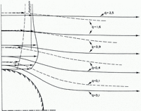
Strain-rates and stresses are given as adjusting polynomials in 1/r, sin θ, and cos θ. They satisfy the equations of incompressibility, of equilibrium and the boundary conditions. The total viscous dissipation rate (which equals U p D, D being the drag) is a minimum only within the class of polynomials which is considered, and Glen’s law is only approximately satisfied. Stream lines so found are given in Figure 2, and normal stresses σ r (for r = R) and σ Ø in Figure 3.

Fig. 2. Stream lines and velocities in the equatorial plane, when a Glen material flows around a sphere without friction and without cavitation. Dotted lines: n = 1 (Newtonian viscosity). Full lines: n = 3. Values of q are in terms of R2U (R – radius of the sphere, U – velocity at infinity). Note the “extrusion flow” when n = 3.

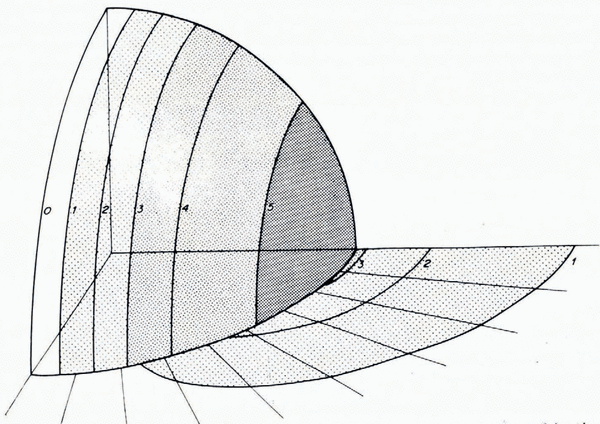
Fig. 3. Underpressure on the sphere and on a meridian plane, taking ![]() as unit. Only one quarter of the sphere is represented. The velocity at infinity is parallel to the horizontal axis of the figure.
as unit. Only one quarter of the sphere is represented. The velocity at infinity is parallel to the horizontal axis of the figure.
In Reference WeertmanWeertman’s (1957) calculation, as well as in the subsequent ones of the present author, there is a confusion between the fluctuating normal stress on the sphere ![]() and its deviatoric part σn′ the only one to produce strain-rates. At the leeward pole, with a Newtonian viscous fluid (n = 1), η being the viscosity:
and its deviatoric part σn′ the only one to produce strain-rates. At the leeward pole, with a Newtonian viscous fluid (n = 1), η being the viscosity:
With a Glen material, when n = 3,

At the upward pole  and σ
0+p
∞ have opposite values. The corresponding drags are, for n = 1:
and σ
0+p
∞ have opposite values. The corresponding drags are, for n = 1:
for n = 3:

The enhancement of the drag with n = 3 comes from the strong enhancement of the fluctuations of σ0. At a large distance from the sphere, the medium behaves as an almost rigid enclosure, and the medium is expelled from the upward side to the leeward side by a “head loss”, at a velocity larger than U
p. With a Newtonian viscous material, this is no longer the case, and the medium is dragged everywhere with a velocity smaller than U
p (see Fig. 2). It can be shown Reference Lliboutry and Ritz(Lliboutry and Ritz, 1978) that the critical value for n which separates both behaviours is ![]()
Weertman’s crude estimation for a cube L
3 was (substituting B by B/3(n+1)/2, since he writes ![]() for a uniaxial pressure, and the effective variables are then
for a uniaxial pressure, and the effective variables are then ![]()

whence, putting ![]() for n = 3:
for n = 3:

The drag was underestimated by a factor 3. This is consistent with the fact that the variations of σ0, which are roughly twice the variations of σn′, were ignored.
Drag of a sphere, taking the melting–refreezing process into account
For a Newtonian viscous body and a sphere it has been found that
The corresponding melting temperature is
Now P K (Cos θ) being the Legendre Polynomials, the harmonic function which takes the value T(R) = A 1 P 1+A 2 P 2+A 3 P 3+… on the sphere and vanishes at infinity is known to be inside the sphere and vanish at infinity is known to be

Since P 1 = cos θ, these expressions reduce to the first term, and we finally find a refreezing or melting velocity normal to the surface of the sphere:

This radial velocity is consistent with a uniform forward velocity of the sphere

Thus in the Newtonian viscous case the motion of a sphere by plasticity and its motion by melting–refreezing are perfectly decoupled. Putting

U = U p+U f with


In the case of a Glen body with n ≠ 1, σn+p ∞ is no longer proportional to cos θ. In T(R), the odd coefficients A 3, A 5,…, do not vanish. Then the sliding by plasticity and by melting–refreezing are no longer decoupled. For large values of R we may write as a first approximation, neglecting the melting–refreezing process:
with k = 4.4 when n = 3. For small values of R. we may write as a first approximation, neglecting the plastic deformation, Equation (41). For the transition size R∗ , for which Up = Uf , both relations are at best only approximate.
Drag of a single hemisphere
Without the melting–refreezing process the flow solution around a sphere is also the flow solution around a hemispherical knob lying on a smooth plane. The boundary condition of no shear stress against the plane is fulfilled. But this is no longer true when the melting–refreezing process is taken into account. The heat sinks and sources which were in the lower hemisphere have disappeared, and new heat sources and sinks have been created in the plane boundary.
If the stresses were the ones calculated without melting–refreezing, the heat-flow lines would have the appearance sketched in Figure 4b. Melting takes place on the plane on the down-stream side of the knob, because (although in the case of a Glen body it is warmer than at infinity), this area is still colder than the nearby leeward face of the hemisphere, where refreezing happens. Thus there is a supply of heat, and melting. On the up-stream side of the knob it is the reverse: there is some refreezing against the plane.

Fig. 4. Sketch of the isothermal surfaces and heat stream lines: (a) around a sphere; (b) around a hemispherical knob.
Thus the two processes of plastic flow and melting–refreezing around a hemispherical knob are not decoupled. This is true even for a Newtonian viscous model of ice. (This point was missed in Reference LliboutryLliboutry (1978).) The numerical solution of the problem would be lengthy, and so the former values of Up and Ut will be kept, as a very rough approximation. It will nevertheless be better than Weertman’s calculation, in which the heat transmission around the knob was ignored: the sliding by the melting–refreezing process was then underestimated by a factor of about three.
Putting

Up = Uf for the transitional size R = R* , and the corresponding value of σ is σ* where

Weertman’s estimation of B1 was 3n = 27 times too large; his estimation of C1 was about 3 times too small. Thus his estimation of R* was about five times too small.
Ubiquity of cavitation with this model
The numerical values given in Table I will be adopted. Then, if U is in metres per year,
Table I. Numerical values of the parameters(1 bar – 105 Pa; 1 year = 3.1557 × 10⁷s)

When there is no cavitation, the normal pressure on the sphere is a minimum at the leeward pole, where it is p ∞—1.34σ. It increases progressively to reach p∞ at the equator (θ =Π/2). Since p∞ = 5 to 30 bar in Alpine glaciers, and in general the sliding velocity is larger than 10 m/year, it follows that ice–bedrock separation must occur in general behind hemispherical knobs a few centimetres high, even without an interstitial water pressure p. Taking this water pressure into account, cavitation becomes ubiquitous in a large range [R1, R2] which includes R *.
In order to calculate the drag in this case, the following new approximations will be made:
-
(1) Instead of a cavity progressively increasing when p increases, a hil-or-miss model will be adopted: no cavitation at all whenp ∞—p = N > σ, and cavitation over the whole leeward side when N< σ.
-
(2) Although the heat sources are consistently changed, the same value of Uf is kept.
-
(3) The stream lines, strain-rates, and stresses on the up-stream side of the knob are assumed to remain more or less the same. Then Equation (44) relating U and σ still holds, σ being defined as a mean over-pressure on the up-stream face of the knob (half-drag on a hemisphere D/4, divided by the cross-section πR 2/2).
It follows that:
-
(a) The extreme values of R for which cavitation stops are the roots of Equation (44), where σ = N and U is a constant:
(46)
-
(b) The total drag (D/2) on a hemisphere with cavitation is
(47)

Friction law over the non-dimensional model
Finally a plane with hemispherical knobs of any size is considered. We assume that they are disposed at random, and that the number of knobs per unit area in the range [R, R+dR] is μ dR/πR3 as long as R 0 < R < R M. It is zero outside [R 0, R M]. The total area which is covered per unit area is then μ ln (R M/R 0). The roughness parameter μ is small enough for the knobs to be considered as independent from each other in the flow problem. The case of superimposed knobs is then uncommon enough to be ignored. If for instance R 0 = 1 μm and R M = 10 m, we need μ ≪ 1/16; we shall see that 1/200 < μ < 1/100 leads to realistic values for the friction.
In order to pass from the case of a single knob to this model, a final approximation or, rather, an unproved assumption is made. In the case of a single knob and no gravity forces the state of stress at infinity was a hydrostatic one. Now, still without gravity forces, we must assume a shear stress τ b at infinity upwards. Then, for a Glen material, the viscosity is no longer infinite at infinite distances, and this may change the whole flow. The question remains open.
With this assumption, the total friction in the interconnected regime (N the same for all cavities) may be obtained summing up the drags π R 2σ for the knobs without cavitation and π R 2(σ+N)/2 for the knobs with cavitation. R is given as a double-valued function of σ by Equation (44) (where U is a constant). Splitting the sum in two at the value σ = σ∗ allows us to integrate by parts. (Weertman’s trick of discretizing the sizes is useless.) For a detailed calculation, the reader may refer to Reference LliboutryLliboutry (1978).
Three distinct cases must be considered:
(1) No cavitation at all
Then

and we finally obtain

where

For n = 3, E(I) = 0.07108, and
or numerically, with the values of Table I, in the metre-bar-year system,
It appears that, in contrast to the Newtonian viscous case (Reference NyeNye, 1970), at small sliding velocities the limiting size R M cannot be ignored. The drag of the large obstacles (R ≫ R∗ ) is not negligible, because σ only decreases like R −1/n .
(2) Cavitation in the range [R 1, R 2]
This happens when

or, numerically, if R M = 10 m, when
Then

and it is found that

For n = 3:

or numerically, in the metre-bar-year system,
(3) Cavitation in the range [R 1,R M]
The cavitation happens up to the largest knobs of the model when N < (U/B
1
R
M)1/n
, that is with the adopted values when ![]() Then
Then

For n = 3

or numerically, in the metre-bar-year system,
On Figure 5, curves of equal (τb /μ) in the (U, N) plane are plotted.

Fig. 5. Friction τ b(U, N) on a plane with independent hemispherical knobs. Non-dimensional model up to RM = 10 m. Numerical values of Table I have been assumed. Weertman’s law holds in the upper left corner, for large values of N. When N = 0, for a given velocity the drag τ b is halved, and for a given drag the sliding velocity U is multiplied by four.
Reference WeertmanWeertman (1964) considers the first case (no cavitation) and the case N = 0 only. Both cases are quite distinct, and the double-valued friction law he found comes from false reasoning, as explained in Reference LliboutryLliboutry (1978).
Friction law over an undulating surface
No cavitation, very small slopes, and Newtonian-viscous ice
Assuming ice to be Newtonian viscous, and no cavitation, this problem has an asymptotic solution for very small slopes which has been given by Reference NyeNye (1969). Only the solution for the two-dimensional case will be recorded here, in the form given by Reference LliboutryLliboutry (1975). Let:

be the longitudinal profile of the bedrock. The wave number ν = 1/λ defined in Equation (5) is related to ω by ω = 2πν, and ωΛ = 2π/Λ. Then dω/ω Λ = Λdν, and a(ω) = b(ν)/Λ has the dimensions of a length. Since b(x) is real, a(—ω) and a(ω) are complex-conjugate quantities.
To obtain the microrelief z 1(x), the low frequencies [—ωΛ, ωΛ ] must be excluded by a perfect filter. There is also a cut-off ω0 for very high frequencies, because the irregularities which are drowned within the micrometric water film are ignored. From Parseval’s theorem it may be shown that the mean quadratic slope of Z 1(x) over a length 2Λ is m1 , given by

The microrelief is non-dimensional in the range [ω Λ, ω0 ] when the contribution of the frequencies [ω 1, ω 2] to m 1 2 is a function of ω 2/ω 1, only. For this it is necessary that
c being a constant independent of the choice of Λ.
Let us introduce a new profile z∗(x), drawn from b(x) by filtering around the transition frequency ω∗(to be defined later) as follows:

Since the terms in Equation (65) outside [ωΛ, ω0] are negligible, it does not matter whether we filter b(x) or z 1(x). The mean quadratic slope of Z ∗(x) over a length 2Λ is m ∗, given by:

For the non-dimensional microrelief
The relation between m∗ and Reference KambKamb’s (1970) roughness parameter is
The first step is to compute the stresses over a pure sine profile z = a p cos ωx ignoring melting–refreezing. Let ωp be the vertical velocity due to plasticity close to the bedrock. The normal pressure against the bedrock is found to be p i+H+p 0 where
(p
0 is the octahedral normal pressure; ![]() vanish against the bedrock).
vanish against the bedrock).
The temperature fluctuation is then –Cp 0, whence a heat flux —(Κ i+Κ b)Cp 0 ω and a vertical velocity owing to the melting–refreezing process
where

Adding the vertical velocity due to plasticity, ωp = – Uapω sin ωx, we find the total vertical velocity when ice at a mean velocity U slides over z = a cos ωx:
whence a = (1 +2η C2 ω 2) a p. Let us define ω∗by
Then

Denoting an average for all x by <>, the mean drag over the bedrock is

According to Equations (73) and (72):

Summing up relatively to dω/ωΛ, the friction over the bedrock z 1(x) is obtained as

No cavitation, very small slopes, and Glen’s law for ice
Reference KambKamb (1970) has estimated the friction for a Glen material, always without cavitation. He starts from the fact that in the Newtonian-viscous case the asymptotic solution over the pure sine profile above gives an effective shear strain-rate
which is independent of x. Summing up for all the frequencies, the effective variables ![]() and
and ![]() are also independent of x. They are a maximum when z = 0.883/ω*. For a non-dimensional bedrock the maximum of the effective shear stress τ is found to be
are also independent of x. They are a maximum when z = 0.883/ω*. For a non-dimensional bedrock the maximum of the effective shear stress τ is found to be
This independency of τ from x should be more or less maintained for a Glen material, and thus in this case η should be a function of z only. It follows, according to Kamb (his detailed development has never been published) that for each Fourier component Equation (68) between p0 and ω p still approximately holds, η having for all the components the same value η m corresponding to this maximum τ m:

(Since the calculation of the stresses in the Newtonian-viscous case is valid only to the first order in a, it is illusory to take into account the average shear stress τ b, which is in a2 , as Kamb does.) The following Equations (69) to (76) still hold, η having the value above. So it is found that
With the numerical values of Table I, in the metre–bar–year system

These relations are much simpler than Kamb’s ones and give more or less the same numerical values in the nine cases which he has studied Reference Lliboutry(Lliboutry, 1975). Discarding his cases 4, 6, and 7 for which, in our opinion, there is cavitation, m* should vary between 0.11 and 0.27, λ* between 0.19 and 0.40 m.
No cavitation, finite slopes
Kamb’s estimation becomes incorrect when the slopes of the microrelief are not very small and Λ/λ* is large enough for the following reason. The strong stresses due to the wavelengths near λ* make ice softer within a layer the thickness of which is of the order of λ*. This layer is unable to make easier the sliding over large bumps, when their height 2|a| is larger than λ*. The largest bumps must make their own “soft layer”, and thus introduce an additional friction. This additional friction will be estimated in the same way as Kamb’s when a pure sine profile is considered.
Almost all the sliding over a large bump is due to plastic deformation and then a p ≈ a. The corresponding effective shear strain-rate is a maximum for ωz = 1. This maximum value is:
When considering a pure sine profile with a large wavelength (

and the drag

Incidentally, let us compare this estimate with the one made in Reference LliboutryLliboutry (1968, Equation (7)) for n = 3, and extended in Reference LliboutryLliboutry (1971, equation (137)) for any n. In these equations a is not the same and must be replaced by 2a.

For n = 3, the present better estimate increases the drag by a factor 1.33. This comes from the variations in the mean pressure σ 0 which were unjustifiably ignored, as said before. The difference is not very large because there is no “enclosure effect” as in the case of an independent knob.
The Fourier-transform technique is unable to solve the plasticity problem for a more general profile, when the slopes are finite. Nevertheless since for a large single sine profile it is |aω|1+1/n which appears in the drag, and not |aω|2 as in Kamb’s treatment, we may suspect that for large wavelengths it is no longer the spectral power density which is the appropriate statistical parameter to consider.
Friction law with cavitation: former approach
Even if the slopes are vanishingly small and the ice is assumed to be Newtonian viscous, the estimation of the friction law over an undulating surface when there is cavitation remains an open problem. Reference KambKamb (1970) suggests that it should be similar to the friction law without cavitation, with a smaller value of the roughness parameter. This is perhaps true in the autonomous regime, which has been shown to be unimportant. In the interconnected regime there is a new variable, p∞–p = N and thus any law of Weertman’s type must be rejected. Variations in the subglacial water pressure p change the sliding velocity very much, a fact which Weertman’s law cannot explain.
In order to tackle this problem a new model of bedrock has been introduced in Reference LliboutryLliboutry (1968) and subsequent articles. The longitudinal profile consists of four superimposed sine curves, with the same value of aω and wavelengths in a geometrical progression of ratio 10
Reference NyeNye (1970) asks “why 31.6?” In order to obtain a realistic spectral power for the displacements, one order of magnitude less would be preferable. The reason is that we wish to eliminate interference between the stress fluctuations caused by each component. The condition of the preceding section must be fulfilled: the nth sine curve must “produce its own soft layer”. Its bumps, of height 2an/π must be larger than the thickness of the soft layer produced by the (n–1)th sine curve, that is λn-1 . Thus one must take:
and realistic values of aω seem to be 0.1–0.2.
The inaccurate value of the estimated drag for a single sine curve afforded an error in the upper limit of cavitating wavelengths by a factor (1.33)3 = 2.35. A more important error was made by putting the same value of N in the drags of each sine curve. Equation (56) in Reference LliboutryLliboutry (1968) is wrong.
With cavitation, the drag over a single sine curve is written:

where s is a function of U and of the size. Let τ 1 and s 1 be the values of Tω and s for the largest sine curve where cavitation happens. Then τ 1 = (aω/2)NΦ(s 1). The mean pressure of ice on the area in contact is P 1 given by
whence
Thus, in order to study the sliding over the next smaller sine curve, N/s 1 must be substituted for N. The drag of this latter sine curve is effective over a ratio s 1 of the total bedrock (over the remainder this smaller sine curve is drowned). Thus:

and so on.
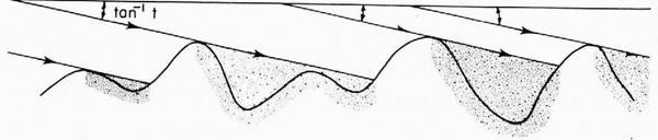
Cavitation over large bumps of similar length and random heights
Let us consider first a large sine profile, for which the melting–refreezing process may be ignored. When cavitation starts, the maximum downward velocity of ice is ω p = Uaω. This happens for p0 = p and sin ωx = 1 in Equation (84), and then

When there are cavities of finite length at pressure p, we may estimate the downward velocity of ice at the roof of these cavities to be the same in terms of N and λ. The slope of the roof of all the cavities is:

In other words we assume that the flow with cavitation is roughly the same on the downstream side of a bump as it would be on a pure sine profile having a maximum slope t, the value of t being such that the minimum value of the normal pressure is N. Experimental work by Reference BrepsonBrepson (1979) has shown that on the up-stream side of a bump the flow is consistently changed, because the general shear affecting the boundary layer concentrates there. Nevertheless the drag may be calculated from the flow on the down-stream side only.
With the numerical values of Table I, in the metre–bar–year system,

When t = aω, the cavitation starts simultaneously in the lee of all the bumps. As t → 0, all the bumps are drowned simultaneously and the friction drops to zero. These circumstancesare very unrealistic. A pure sine profile is not a good model for roches moutonneées. A model where the maximum leeward slopes and the height of the bumps fluctuate in a random way must be preferred. If the bumps are of similar length λ, the slope of the roof of the cavities t should be always given by Equations (93)–(94). The lengths of the cavities differ from one another, but t is the same for all.
The friction law depends on the distribution of the heights and leeward slopes, which is completely unrelated to thespectral power density. As already suggested in Reference LliboutryLliboutry(1968) it is convenient to introduce instead the shadowing function s(t). This function, which is defined on Figure 6, has already been introduced in the study of the reflection of solar rays and radar waves on rough surfaces Reference Smith(Smith, 1967). Here s(t) is the part of the bedrock which is in contact with moving ice (the water film of micrometric thickness being ignored).

Fig. 6. Definition ofthe shadowing function. s(t) = (area of the shadow)/(total area).
The normal pressure on the bedrock is p where a cavity exists, and p+P(x) where there is contact (P(x) > 0). Let ![]() denote a mean value for all the area with contact. According to Equation (90):
denote a mean value for all the area with contact. According to Equation (90):
Since a uniform pressure p on the bedrock affords no drag, the friction is:
The ice limit goes down as much as it goes up, and then:
For very large cavitations, z’(x) is more or less constant over each small area where there is cavitation and P(x) is significant. Then:
whence
For small cavitations P(x) is in general less where z’(x) is negative, and then ![]() is larger than
is larger than ![]() . This introduces an additional term, the only one to subsist when no cavitation occurs. This term will be estimatedin the case of a pure sine profile.
. This introduces an additional term, the only one to subsist when no cavitation occurs. This term will be estimatedin the case of a pure sine profile.
When there is no cavitation, Equation (93) may still be used to define a function t, which no longer has any physical meaning.,

For a large pure sine curve, where the melting–refreezing process is negligible, the friction τω is then given by Equation (85) so that
Comparing Equations (100) and (101) it follows that

Let us introduce the mean quadratic slope m. For a pure sine profile ![]() Putting
Putting

Equation (102), which is valid when s = 1, becomes:
Since the additional term must vanish for large cavitations (s ≪ 1), the value from Equation (104) will be adopted after multiplication by s β (β > 0). In Reference LliboutryLliboutry (1978) the friction over a large pure sine profile has been estimated to be:

Over a sine profile:
sin ωxc = T has been calculated in the aforementioned article as a function of s (equation (9)). As shown in Table II the very elaborate function Φ/2 is more or less the same as the much simpler one obtained with β = 2:

Table II. Functions relative to a pure sine profile

This function, that will be called the friction function, will be adopted in the more general case, for any degree of cavitation or no cavitation. The friction over irregular large bumps of similar length is thus estimated to be:

For a pure sine curve F(T), which is plotted in Figure 7, increases suddenly when cavitation starts, and drops to zero at very large cavitations. For bumps of irregular height it is no longer valid.

Fig. 7. Friction function F(T) forn periodic bumps. m is the mean quadratic slope, λ the wavelength (in metres), U the sliding velocity (in m/year), N = p∞–p (in bars), τb the friction (in bars). The figures along the curves are the values of s(T).
Let us consider the case of a Gaussian distribution of the displacements z(x) and the slopes z’(x). (We shall say that the profile has a Gaussian modulation.) Smith has calculated that in this case:

To obtain this result Smith also assumes a negligible self-correlation, but it has been shown by Reference Benoist and LliboutryBenoist and Lliboutry (1978), by numerical simulation of random profiles, that s(T) is practically insensitive to this last assumption.
The corresponding friction function is also plotted on Figure 7. It has a completely different shape from that for a sine curve. When the cavitation is significant F(t) ≈ 0.54 within a few per cent. For very large cavitations F(t) increases a little, up to F(0) = ![]() = 0.5642, instead of vanishing.
= 0.5642, instead of vanishing.
A more realistic model
In order to model the most general undulating bedrock we must consider:
-
1. Very large undulations where no cavitation occurs at any realistic velocity. They afford a small drag τ 1 which, since only plastic sliding is involved, is proportional to U 1/n . The choice of the cut-off wavelength A affects this drag. Assuming that the largest undulations are considered as part of the microrelief or as part of the smoothed reference profile, the corresponding dragenters into the local friction law or into the expression of the friction in terms of the body variables (Equation (2)).
-
2. Large bumps where cavitation may happen which are superimposed on the very large undulations. Assuming that they are of similar length they afford the drag calculated above (Equation (107)) where N = p ∞—p has a local, fluctuating value. The overburden p ∞ is larger on the up-stream side of a very large undulation, and smaller on the down-stream side, by more or less the same amount. Since the drag of the cavitating bumps, say τ 2, is roughly proportional to N, these fluctuations cancel each other.
-
3. Still superimposed on the cavitating bumps, smaller undulations. Only the ones which lieon a ratio s of the total area afford a drag, the other ones are entirely drowned (s is the shadowing function for the cavitating bumps above). Since the mean normal pressure where moving ice and bedrock are in contact is N/s, cavitation seldom happens on these small undulations. The corresponding dragτ3 then follows a Weertman’s law in U 2/(n+1).
The total friction over this composite model is
κ1 and κ3 being constants, and m 2 the mean quadratic slope of the cavitating bumps alone.(110)

According to Equations (100) and (103), U is proportional to,N n/T. The third term is then proportional to N 2n/(n+1)[s(T) T −2/(n+1)]. This last factor within brackets, with n = 3, has been plotted on Figure 8. At very large cavitations it remains finite in the case of a sine profile, and vanishes when a Gaussian modulation is introduced. Thus whenN is zero, the only drag which remains is the small one in U 1/n introduced by the very large undulations.

Fig. 8. Values of S /T
Conclusion
The analysis which has been done shows definitely that the local friction law is strongly dependent upon the geometrical model of bedrock which is assumed.
In the case of independent knobs lying at random on a plane, the frictionτb may be estimated by Equations (49) to (60), which are plotted on Figure 5. These relations have been calculated with hemispherical knobs, but their precise shape is unimportant when one considers the many approximations and rough estimations which are introduced into the theory all the way along. For very large values of p ∞—p = N (very thick glaciers with subglacial waterways at atmospheric pressure, a rare circumstance), Weertman’s law is valid, with a largely modified numerical factor, and a small correction to account for the limiting size R M. Otherwise N enters into the friction law because the ice–bedrock interface cannot be absolutely watertight and the interconnected hydraulic regime predominates. With increasing values of the subglacial water pressure p, the friction lowers progressively to one-half of the former value.
This last value is reached for p = p ∞, N = 0. Locally, and during a short time, N can even become negative, a fourth case which has not been considered in this article. The drag then lowers a little more. It may be shown that, in order to have no drag at all. N must reachthe value —σ*, given by Equations (45) and (45’), which is totally unrealistic.
In the case of interfering bumps, the friction law without cavitation is given by Kamb’s simplified relations, Equations (80)–(82), for vanishing slopes only. Nevertheless, even with finite slopes, Weertman’s law in U 2/(n+1) holds as long as no cavitation appears. With cavitation, the friction law cannot be calculated with accuracy. Fourier analysis becomes useless. It is the shadowing function s(t) which gives the pertinent information about the micro-relief. Now, the shadowing function of a pure sine profile is a very peculiarone, and the friction law on such a model is accordingly a red herring. Periodic bumps with a Gaussian distribution of the heights and slopes have a quite different shadowing function, and afford a quite different friction law, plotted in Figure 7.
For any undulating surface, even taking into account smaller superimposed undulations, the drag almost vanishes with N. The only drag for N = 0 comes from the largest undulations and varies as U 1/n . The difference from the case of independent knobs is noteworthy.
It thus seems possible to assess the relative input of isolated knobs and of undulations into the drag by monitoring the seasonal fluctuations of the sliding velocity and of the subglacial water pressure p.
If we assume now that N is given, with independent knobs there is a single value of U for each τb , contrary to Weertman’s assertion. With undulations,U may be a multivalued function of τb or not, according to the shadowing function and to the relative importance of the different kinds of drag. These conclusions are of course essential for the study of kinematic waves, glacier surges, or glacier falls (ice avalanches). Nevertheless, as said in the first section, the introduction of these local friction laws into glacier dynamics is not simple and straightforward. Several models may be assumed for the pressure p w in the waterways. In our opinion it is useless to tackle this problem without having a particular case in view and the pertinent field measurements to hand.
Discussion
B. Ladanyi: The friction law for the ice–rock interface you have shown takes into account, in fact, only viscous friction, and not the true friction in Coulomb’s sense. However, Coulomb friction might be present at the interface because of the presence of rock debris, and also because of possible brittle fracture of ice in the vicinity of obstacles. Do you not think that it would be useful to modify the basic Glen’s flow law so that it takes into account the effect of the hydrostatic component of the stress tensor on the creep-rate, which would lead to a more realistic friction law for the interface?
L. A. Lliboutry: I agree with your first two sentences, not with the third one. Coulomb’s law is the normal friction law for an almost perfectly plastic solid, that is when n in Glen’s law is very large. For this case the cavitation is extremely well developed, the contact area is proportional to the normal pressure N, and the local friction over this contact area a constant. Thus the mean friction becomes proportional to N as a consequence of cavitation, not of any influence of N on the creep law.
J. Weertman: The language problem has led to two misunderstandings that are repeated in your many papers about what I have stated in my papers. (1) I have never claimed that glacier beds are watertight. In fact, in all my papers that deal with basal water I quote Dr W. H. Ward that the contrary is true. (2) Although I pointed out (as of 1972) that there is a dearth of descriptions of extensive Nye networks in the literature, I did not use this lack to claim that Nye channels do not exist.
Lliboutry: “Watertight” must be understood according to the context. When saying that, in your opinion, the ice–bedrock interface (not the bedrock) should be watertight, I refer to your paper in Reviews of Geophysics and Space Physics, 1972. You demonstrate there that water cannot drain into subglacial R-channels. This is true when ice slides over a perfectly plane and smooth surface. Actually on bedrock there are glacial striae, rock joints, areas and stripes of previous drift, etc., where your reasoning does not hold. When these are not exactly in the direction of flow, ice cannot enter by plasticity into these millimetric channels, sliding is too fast. Viscous heat dissipation within the micrometric water film and geothermal heat should prevent most of these millimetric channels from being obstructed by regelation ice.
By the way, I see no reason to call these already well-known and described features “Nye channels”, the more so as Nye only reproduced my point of view (Reference LliboutryLliboutry, 1968, p. 55).