


Introduction
Large floating ice shelves surround much of Antarctica. Their fast flow, often in excess of 1000 m year−1, is of tremendous interest in the study of ice dynamics and Antarctic climatology. On the one hand, ice-shelf dynamics are controlled by both the ocean and the atmosphere. On the other hand, because of high ice velocities, ice shelves involve time-scales which are ten times smaller than those involved in the grounded inland ice sheet (typically a few hundred years for an ice shelf versus several thousand years for a grounded ice sheet), These considerations suggest that ice shelves should be the first elements of the ice-sheet system to respond to climate changes. Furthermore, their involvement in climate instabilities such as Heinrich events is also conceivable.
Early analytical studies of ice-shelf flow (Weertman, 1957) were one-dimensional and the role of lateral boundaries was not clearly taken into account. Despite the simplicity of this early work, it generated an awareness of the interactions between an ice shelf and a grounded ice sheet, and led to the discovery of an instability mechanism, since known as the marine ice-sheet instability, which could occur in the grounding zone. Thomas (1973a, b) developed an approximate solution for an ice shelf in a rectangular channel, in which the friction at the sides was parameterization using observations on the flow of the Brunt, Ross and Amery Ice Shelves. The first two-dimensional computational study is due to MacAyeal and Thomas (1982), who solved the stress equations using the finite-element method. Some other numerical models using the finite-difference method (Determann, 1991; Huybrechts, 1992; Jonas and others, 1994) have since followed. The work we present here is in keeping with the spirit of these previous studies: the zeroth and the first order of the Stokes’ equations, heat transfer and mass conservation are treated simultaneously.
Ice-Shelf Dynamics
a. Diagnostic equations
First, we shall derive the Stress-equilibrium equations using simplifications made possible by some of the features of an ice shelf. These partial differential equations, as well as their boundary conditions, have not yet been universally accepted. The derivation we present here is basically the same as that proposed by MacAyeal and others (1986), also known as the “reduced” model of Morland (1987), but we give a different description based on the force balance over an elementary column.
By considering the typical geometry of an ice shelf, we can recognize an obviously small parameter, known as the aspect ratio, which is the ratio of the ice thickness (H) over the horizontal scale (L). For the Ross Ice Shelf, L is about a 100 km and H is less than 1 km. Appropriate recognition of the smallness of this aspect ratio will allow us to make assumptions similar to the quasi-geostrophic approximation in meteorology (in which the smallness of the Rossby number is used). Since acceleration, inertia terms and Curiolis force are neglected, the Stokes’ system can be written as
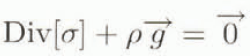
where g is the gravity acceleration, ρ is the ice density and [σ] is the stress tensor. For our specific problem, we shall use a vertically integrated formulation of this system. Therefore, we consider an elementary column through the ice shelf (see Fig. 1) of dimension δx, δy and H; the upper boundary is in contact with the atmosphere, whereas the lower one is in contact with the ocean. We assume δx and δy small and of the order of H. The force budget on this column is

where F is the force, [σ] is the stress tensor averaged over the elementary surface which is considered and m is the ice mass of this elementary column. The index is related to the surface, where the force or tensor is applied (see Fig. 1). The surface vectors, S i are pointing out ward and the upper and lower boundary conditions are the following:

where l w is the sea-water density and z b the ice-shelf base elevation. The upper surface is stress-free (the friction of winds and atmospheric pressure are neglected) and the bottom is just subject to water pressure. The projection of Equation (2) on the x-horizontal axis, using Equation (3) (note that here x and y have the same role, and we shall only write the x projection for the sake of brevity) leads to

We can now use a Taylor’s expansion of the first order, which yields

Note that from now on the stresses are averaged over depth. A vertical integration of the Stokes’ system, taking into account the upper and lower boundary conditions and using differential calculus and the Leibnitz’ rule would have led to exactly the same result (MacAyeal, 1994). We emphasize that the derivation described above has nothing specific to do with the finite-difference method described in the following part. Note also that no assumption resulting from the smallness of the aspect ratio has been made yet.

Fig. 1. Schematic view of an ice shelf showing the force budget on an ice column and the different notations (axis, surfaces …).
Actually, in Nature, strain rates and velocities are much easier to measure than stresses, and the next step in the calculation will be to write Equation (5) in terms of strain rates. Here, we make the assumption that ice is an isotropic material and write the strain-rate tensor as
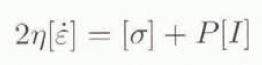
where η is the ice viscosity (which depends on temperature and on the second invariant of the strain-rate tensor, cf. sub-section c below),

One of the major features of ice-shelf dynamics, and what makes them completely different from grounded ice sheets, is the independence of strain rates with depth. An elegant demonstration is not derived here but it follows from the small-aspect ratio which we discussed at the beginning of this section. A rigorous approach (MacAyeal, 1989) leads to the following result: ∂ε xx /∂z, ∂ε xy /∂z and ∂ε yy /∂z are of order αU/L 2 (α being the aspect ratio, U the horizontal velocity scale and L the horizontal scale). By a similar reasoning, the first two terms in Equation (7) (horizontal gradients of vertical shear stress) can be safely disregarded. The ice density is assumed to be constant in the whole ice shelf and thus ice thickness should be interpreted as an “ice-equivalent” thickness. The upper boundary condition (Equation (3)) is accounted for, and Equation (7) then simply becomes

where we have used the ice incompressibility. We are now able to rewrite Equation (5) using Equations (6) and (8) and the assumption that the ice shelf floats in local hydrostatic equilibrium,

The vertically averaged viscosity which appears in this equation comes from the vertically averaged stress components in Equation (6). An x and y permutation in Equation (9) would lead to the y projection of the vectorial expression in Equation (2). One ran notice that these diagnostic equations are different from those described by Jonas and others (1994), Determann (1991) and Huybrechts (1992). This difference arises from the doubtful assumption at the outset of their reasoning, that ∂σ xz /∂z, which is actually of the same order (order 1) as almost every other term of the Stokes’ system, is supposed to be negligible. Weertman (1957), Thomas (1973a) or Sanderson (1979) had this term in their early studies but the mistake probably arose from a misunderstanding of the paper of Sanderson and Doake (1979): “Is vertical shear in an ice shelf negligible?”.
We now have a system of equations which computes the velocity field from the ice thickness. This set of partial differential equations can be solved numerically using a finite-difference scheme, as described below.
b. Boundary conditions
Strictly speaking, the major assumption of the previous reasoning (the independence of strain rates with respect to depth) is not valid near the boundaries. For instance, the grounding line can be a transition zone where the flow changes from a vertical shear-stress regime into a longitudinal-stress regime. This problem, probably one of the most interesting in ice-sheet modelling, has been treated analytically by Barcilon and MacAyeal (1993) for a Newtonian rheology and numerically by Lestringant (1994), in both cases for two dimensions. Here, we chose to lake only the “far field”’ into account, meaning that the boundary condition is applied far enough from the grounding line, or from the ice from where the same kind of problem occurs (Morland, 1987).
Boundary conditions in mechanical problems often split into two types: kinematic (which means that the velocity is specified on the boundary) or dynamic (the force is specified). This distinction is in fact artificial and depends upon the domain. Since sliding on the sides is not well understood, we chose to describe it with kinematic boundary conditions (zero velocity). This is consistent with observations on large ice shelves, for instance, on the Ross Ice Shelf along the Transantarctic Mountains, but a further parameterization of sliding is necessary for smaller scales. In sonic cases such an approach lends to over-estimate the restraint (MacAyeal and others, 1986). The ice inlets (glaciers and ice streams) are also naturally described with kinematic boundary conditions: their velocities are parameters of the model. On the other hand, the ice front is typically a dynamic boundary condition: the horizontal longitudinal stress in the ice has to be balanced by the water pressure. Following the vertically integrated approach above, for an ice front parallel to the y axis the force balance on the front can be written formally as

Equation (10) is a vectoral expression that we shall project on the x and y axes; using the pressure from Equation (8):

Note that the similarity between the diagnostic Equation (9) and the boundary condition (Equations (11)) provides a rather good argument for the self-consistency of this method. No assumption about the “confinement” of the flow at the ice from is made unlike the works of Determann (1991) or Huybrechts (1992).
c. Ice rheology
The previous analysis is valid for Stokes’ flow of any floating isotropic material. In this work, ice is assumed to follow Glen’s flow law (Paterson, 1994):

where A T is a coefficient dependent on the temperature (Arrhenius’s law), τ is the second invariant of the deviatoric stress tensor and ε is the second strain-rate tensor invariant. The exponent of Glen’s flow law (n) is assumed to be equal to 3. We need the depth-averaged viscosity and A T −1/3 since the strain rates are independent of depth. The temperature is numerically computed by solving the time-dependent heat equation: the temperature evolution at a fixed point in space (Eulerian description) is determined by vertical heat diffusion, horizontal heat advection and vertical heat advection so that

where T is the temperature, t is the time. u, v, and w are the components of the velocity, c is the specific heat capacity and K is the thermal conductivity.
d. Time evolution: the prognostic equation
All the time-dependent terms in the Stokes’ system have been neglected (see Equation (1)). The time evolution is thus determined by mass conservation in a column

where u is the horizontal velocity field, a is the sum of the surface and bottom accumulation and divH is the horizontal divergence.
The Numerical Scheme
Solving the model equations using a computer requires discretization on to a numerical grid. The equations described above (diagnostic equations, boundary conditions, heat and mass conservation) are discretized on to the regular staggered grid shown in Figure 2. In other finite-difference studies, viscosity gradients in the diagnostic equations are neglected, mostly because they often induce wiggles in the results. On the other hand, in MacAyeal’s finite-element works, because of the method itself, the ice viscosity is a piecewise constant function over each triangular element: grid refinements are needed near boundaries and where gradients are important. The resolution scheme we present here takes viscosity gradients into account, is numerically stable, and avoids the formation of wiggles. The discretized form of Equation (9) is:

The second equation (y projection) is obtained by x and y, u and v, i and j permutations. By ordering u i,j and v i,j in a single-column vector U and by using a similar discretization for the boundary conditions, we build a set of 2N (N being the number of grid points) non-linear equations with 2N unknowns, where
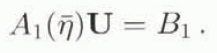
This system can be linearized using a Newton–Raphson method, though a simple successive-approximation iteration (or Picard iteration) over the viscosity leads to satisfactory convergence. This means that Equation (16) is solved as a linear system by Gaussian elimination, until convergence of the velocity field. This computation is performed using a sparse-matrix algorithm (Duff and Reid, 1979).
The solution of the heat equation is derived from the method used in a grounded ice-sheet model (Fabre and others, 1995). We use an implicit scheme in time and an upwind scheme for the horizontal advection. There are some specific treatments for the ice shelf: (1) The basal boundary condition is fixed at the freezing temperature of sea water. (2) As far as the vertical advection is concerned, it follows from the independence of strain rates with depth that the vertical velocity varies linearly with depth. Its value at the ice-shelf bottom depends significantly on the melting (or refreezing) rate, thus affecting the temperature profile. In future, basal melting should be taken into account but in this article we only consider simplified examples, thus we assume no melting or refreezing. Our model cannot be used to compute the temperature profile at the grounding line, as it depends strongly upon the temperature field in the grounded ice sheet. Here, since the temperature does not alter qualitatively the results, we chose to neglect horizontal heat advection at the grounding line where the temperature profile is then computed analytically (Robin, 1955).

Fig. 2. Numerical grid used in the model.
It is important to notice that the mass-conservation equation cannot be written as a diffusion equation in ice shelves. This feature is probably the most difficult technical aspect one encounters when trying to adapt a grounded ice-sheet model to an ice-shelf application. A classical semi-implicit discretization is used here and a linear set of N equations with N unknowns is to be solved:
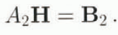
B 2 is a column vector of dimension N, H is a column vector containing the thicknesses at each grid point and A 2 is a N by N matrix which has five diagonals (tridiagonal with two fringes). Adjustments on the time step are performed to maintain numerical stability and to build a matrix (A 2) with a dominant diagonal. This system can therefore be solved by point relaxation (Press and others, 1986). This scheme is numerically stable and does not require smoothing.
Table I. Input parameters for the ice-shelf model

Results on various simplified geometries
The numerical model has been applied on the following simplified geometries (see Fig. 3):
-
A rectangular channel.
-
A slightly divergent bay.
-
The same divergent bay with a small pinning point (island of 200 km2) in the middle.
A freely expanding ice tongue has been added beyond the confined ice shelf in order to test the model (see the following part: testing ice-shelf models). A similar exercise has been performed by Sanderson (1979) in a one-dimensional study. One of his most interesting results was that an ice shelf could not survive in a strongly divergent bay (indeed cavitation, i.e. hole in the ice shelf must occur if the angle is not acute enough). Following Sanderson’s criterion, the divergence of the bay in our second example is not strong enough to produce cavitation and we therefore assume that the ice shelf remains in contact with the sides of the bay.
The model is run from a 1 m thickness (except at the grounding line) to a steady state after 5000 years and we use the results to estimate the force budget in the ice shelf.
Table 1 summarizes the different input parameters used for the model. The aim of this paper is to show, in a simple manner, the applicability of our ice-shelf dynamics formulation and the role of pinning points. This is why many input parameters are assumed to be constant, whereas in Nature they can vary significantly.
A pictorial representation of the major features of the results (for the slightly divergent bay) is shown in figures 4 and 5. As observed in Nature, the ice shelf is thinner and faster flowing near the ice front. A small oscillation in the thickness field occurs at the junction between the freely expanding ice tongue and the embayed ice shelf, due to the strong singularity of the corner. This wiggle, which is not a grid-point to grid-point oscillation, probably comes from the inability of the numerical model to treat the singularity. The temperature gradient is stronger near the base than near the surface: this is a typical shape when one does not consider basal melting or accretion. This implies that, in our particular examples, because of the vertically integrated form of the equations, the dynamics are controlled by the upper layers of ice, which are colder and thus more viscous.
An ice shelf is naturally “pulled” seaward tinder the action of the difference of density between ice and sea water in which it floats, and a restraint is exerted by the sides of the bay, islands and ice rises. This restraint (known as the back force) can be computed by comparing the simulated stress tensors to the theoretical stress distribution for a freely expanding ice tongue as defined by Weertman (1957). The hack force for the three different kinds of bay are plotted in Figure 6. One notices the huge restraint (almost half of the total restraint) exerted by the small island. The role of the angle of divergence on the back force is also significant (of about 5000 GN).

Fig. 3. The three oversimplified geometries which are considered in this work: a channel (a), a divergent bay (b), and a divergent bay with a small island in the middle of the flow (c).

Fig. 4. Thickness (upper panel) and velocity field for the slightly divergent bay, as a result of the model: the velocity-field contours are given even 100 m a−1 and the maximum velocity is 1400 m a−1.

Fig. 5. Computed temperature profiles on the centre line (symmetry axis) for the slightly divergent bay.
Figure 7 shows that the effect of an island (and of the divergence of the bay) on the thickness field must be taken into account. This will be of special interest in future models that will couple ice sheets and ice shelves and evaluate the position of the grounding line.
Testing Ice-Shelf Models
The first concern of the modeller should not be to fit the data but rather to build a self-consistent tool. This means that a “bad” model should not be rejected due to disagreement with reality bin rather because of its inability to conserve physical quantities. Only then, it can be compared with observed data. Here, we propose three exercises that can be easily coded to test an ice-shelf model.

Fig. 6. Back force computed for each geometry: channel (full line), divergent hay (dashed line) and divergent bay including an island (dotted line). The rough aspect of the curves associated with the divergent bay is an artifact due to the discretization, specific to the finite-difference method.

Fig. 7. Thickness along the centre line for each geometry (the thickness is set equal to zero at the island).
1 Mass conservation
When in steady state, mass flux out should equal mass flux in.
2 Divergence theorem
The divergence theorem described below reflects a simple concept: the action–reaction principle. The integration of a horizontal projection of the Stokes’ equations over a defined volume (v) is zero:

Mathematical manipulations on the divergence operator of Equation (18), combined with the divergence theorem, lead to
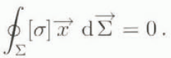
In the “added” ice tongue, because of the lack of horizontal shear stress at the lateral boundaries, this theorem can be used to verify the numerical computation. In the embayed ice shelf, the same theorem can be applied to determine the back force: indeed, if we define the closed surface (Σ) by x = x 0, the upper and the bottom surfaces of the ice shelf, the ice front, the sides of bay and the island boundary, the [σ]x dΣ quantity can be evaluated easily everywhere except around the island and along the lateral sides, The restraint due to the lateral sides and the island (back force) is thus obtained by a simple subtraction, since we know that the sum of these quantities has to vanish as in Equation (19).
3 Energy conservation
For the sake of simplicity in the equations, the following test is only valid for an idealized ice shelf without any accumulation at the surface and at the bottom. The test is a little more complex if we have ice fluxes through the upper or lower boundaries.
The sum of the work done by each exterior force is equal to the kinetic energy increase added to the sum of the work needed to deform each element of the system. For a steady state (no time derivatives), we have

where ![]() is the ice velocity vector. One can recognize the heat production due to ice deformation on the lefthand term of the previous equation.
is the ice velocity vector. One can recognize the heat production due to ice deformation on the lefthand term of the previous equation.
By dividing the boundary surface into three parts: the kinematic boundary with a zero velocity field (Σ3), the kinematic boundary at the grounding line (Σ1) and the dynamic boundaries — ice front, the upper and lower boundaries (Σ2) —, the previous expression can be simplified, because

and therefore

Table 2 summarizes the results of the different tests: the numerical model seems to conserve mass and to verify the divergence theorem in a satisfactory way (about 1% of error for each geometry). The energy test is much worse (a 7% error) but a great part of this error may be due to the treatment of the results of the model itself. Indeed, the integral over the entire volume in the first member of Equation (22) is difficult to compute and truncation errors are hence much more important than in the other tests.
Table 2. Summary of test results

Conclusion
The first EISMINT experiment (Bremerhaven, June 1994) on ice-sheet and ice-shelf modelling proposed by R. Hindmarsh has shown that a special effort was needed for ice shelves. In particular, every model had difficulties in conserving mass. Some of these difficulties were probably inherent to the problem itself, and others occurred because an agreement on how to formulate the equations had still to be achieved. We have presented here a finite-difference version of MacAyeal’s model, including a heat-transfer computation and a few tests to show the self-consistency of the model. Furthermore, such a model can be used to evaluate the evolution of the back force associated with climate changes and it thus appears as a useful tool to study the West Antarctic ice-sheet dynamics. The same model is applied to the Ross ice-shelf geometry in a companion paper (this symposium).
Acknowledgements
We should like to thank sincerely Professor D. R. MacAyeal for having hosted V. Rommelaere during 3 months at the University of Chicago. V. R. also thanks Professor V. Barcilon for very helpful discussions; especially the “energy test”, which was widely inspired from these discussions. A student-travel grant was provided by the European Science Foundation in the framework of EISMINT. This work was supported by CNRS (PNEDC). The graphics were produced using the GMT (Wessel and Smith, 1991) software.


