Quantitative Airborne Inventories in Dense Tropical Forest Using Imaging Spectroscopy

Abstract

Tropical forests have exceptional floristic diversity, but their characterization remains incomplete, in part due to the resource intensity of in-situ assessments. Remote sensing technologies can provide valuable, cost-effective, large-scale insights. This study investigates the combined use of airborne LiDAR and imaging spectroscopy to map tree species at landscape scale in French Guiana. Binary classifiers were developed for each of 20 species using linear discriminant analysis (LDA), regularized discriminant analysis (RDA) and logistic regression (LR). Complementing visible and near infrared (VNIR) spectral bands with short wave infrared (SWIR) bands improved the mean average classification accuracy of the target species from 56.1% to 79.6%. Increasing the number of non-focal species decreased the success rate of target species identification. Classification performance was not significantly affected by impurity rates (confusion between assigned classes) in the non-focal class (up to 5% of bias), provided that an adequate criterion was used for adjusting threshold probability assignment. A limited number of crowns (30 crowns) in each species class was sufficient to retrieve correct labels effectively. Overall canopy area of target species was strongly correlated to their basal area over 118 ha at 1.5 ha resolution, indicating that operational application of the method is a realistic prospect (R² = 0.75 for six major commercial tree species).

1. Introduction

Tropical forests are a major terrestrial plant biodiversity reservoir [1]. The preservation of this biome is therefore globally important. Persistent deforestation [2] is resulting in drastic declines in biodiversity. From 2000 to 2010, logging in natural forests removed approximately 5% of the world’s forest area [3]. While the biggest drivers for biodiversity change [4] have been shown to be land use change and climate change, logging impact on the biodiversity of various taxonomic groups (mammals, birds, amphibians) is also well documented [5]. Logging impact is not restricted to the removal of a few commercial stems per ha, but also includes damage associated with opening tracks to access to the logging area. Untargeted trees can be wounded in the process of timber felling and hauling, contributing to carbon release [6] and possibly slowing forest recovery rate [7] by favouring fast-growing species such as lianas [8,9]. Logging may therefore profoundly modify the floristic composition of the exploited plot [10] while disturbing wildlife [11,12]. Proper management of tropical forests is therefore crucial to mitigate the erosion of biodiversity [13].

Remote sensing technologies can provide valuable information for the preservation of tropical forests. Large-scale species distribution maps may provide valuable insights into species autecology and species population dynamics. Imaging spectroscopy has proven useful in monitoring the development of invasive species [14,15,16]. From a forest management perspective, evaluating abundance and spatial distribution of commercial species will help prioritize areas to be set aside for regeneration purposes and biodiversity conservation, or simply because there is not enough commercially valuable resource for logging operations. Accurate mapping of species prior to opening roads and tracks can therefore support the development of reduced impact logging techniques by minimizing the detrimental impact on soil and forest cover and contributing to protect and maintain forest diversity [17]. This technology is particularly well adapted to tropical forestry, since trees of commercial interest are typically large, upper canopy trees (dominant or emergent) but making up a small part of the entire tree community.

The efficacy of tree species discrimination in tropical forests via airborne imaging spectroscopy has been demonstrated [18,19,20,21,22]. At leaf scale, part of the SWIR1 domain (1467 nm to 1771 nm) was found to support accurate species identification. The SWIR2 domain (1994 nm to 2435 nm) was also found to be important in discriminating species at crown level [23]. A study conducted in semi-deciduous tropical forest [24] reported that including SWIR information (1045 nm to 2395 nm) improved their classification accuracy from 64.2% to 79.8%. While extending the spectral range increases the discriminative power of hyperspectral imagery, it has known drawbacks. Sensors limited to the VNIR domain are lower cost, more widespread, more easily miniaturized to mount on UAV platforms and have better intrinsic performance (higher signal-to-noise ratio). Hence, the balance between costs and benefits of increasing the spectral range should be assessed with respect to the specific task considered.

Improved accuracy has been reported from performing classification at the crown level as opposed to the pixel level [22,25,26]. However, segmentation of individual tree crowns (ITCs) in dense canopies remains a difficult task. Light detection and ranging (LiDAR) can help considerably. A recent benchmark study comparing crown segmentation methods using the LiDAR point cloud of a dense tropical canopy [27] identified AMS-3D (Adaptive Mean Shift in 3 Dimensions) as the most effective method. LiDAR and hyperspectral data fusion may further improve our ability to distinguish individual crowns [28].

Most studies in tropical forest so far have focused on discriminating a limited number of species against one another. In the present study, we are interested in retrieving a few target species amongst a very large number of non-focal species. To this end, one might consider focussing the annotation effort on the well-known more easily recognized focal species. This raises the question of the definition of the non-focal species class. A random sample of pixels of the area may capture the diversity of species in the background but will most likely include pixels of the focal species as well. Standard measures of accuracy such as F-measure then become inappropriate during the training stage due to this possible source of bias. A new unbiased criterion was proposed to replace the F-measure in such settings [29] It is based on the evaluation of the focal class (given by the recall metrics) divided by the probability that a sample is classified in the focal class among the non-focal class. This methodology was applied to identify five species on Barro Colorado Island (BCI) [19]. In the latter study, the authors did not specifically study the sensitivity of the classifier to the level of bias (impurity of the non-focal class).

Finally, we go beyond individual tree classification accuracy evaluation by exploring how well one can predict the cumulative basal area of commercial species per unit area from imaging spectroscopy to truly tackle the issue of quantitative forest resource mapping.

Our study starts by examining the benefits of using a SWIR sensor (1000 nm to 2500 nm) in conjunction with a VNIR sensor (400 nm to 1000 nm) for tree species discrimination. We then move on to the core of our study, which is to evaluate the potential of hyperspectral imagery in an operational setting. We first explore for 20 locally abundant species how much the retrieval rate may depend on the diversity of the set of species among which the target species are mixed. We compare the performance of different binary classifiers developed to retrieve target species from wide views of the forest canopy after delineating individual tree crowns using LiDAR data. We further examine the impact of mislabeling of the focal and non-focal classes on the different classifiers’ performance. We also briefly examine the impact of the size of the training set representing the species of interest. We finally compare hyperspectral predictions of basal area per species to a large ground inventory database.

2. Materials and Methods

2.1. Study Site

The study site of Paracou (5°18′N, 52°53′W) was established during the 1980s in French Guiana. The main objective of the experimental set-up was to document the impacts of different silvicultural practices on the dynamics of a tropical rainforest in order to provide guidelines for its sustainable exploitation [30]. Seventy-six 125 × 125 m plots (118.75 ha) are regularly monitored (stem girth and vital status being recorded). All trees with a diameter at breast height (DBH) higher than 10 cm have been identified to species level (or higher order taxon level if species was unknown). At the onset of the experiment, all the trees were geo-located using a meter tape after materializing a 12.5 × 12.5 m grid on the ground using strings. Tree location accuracy was estimated to be +/− 2 m.

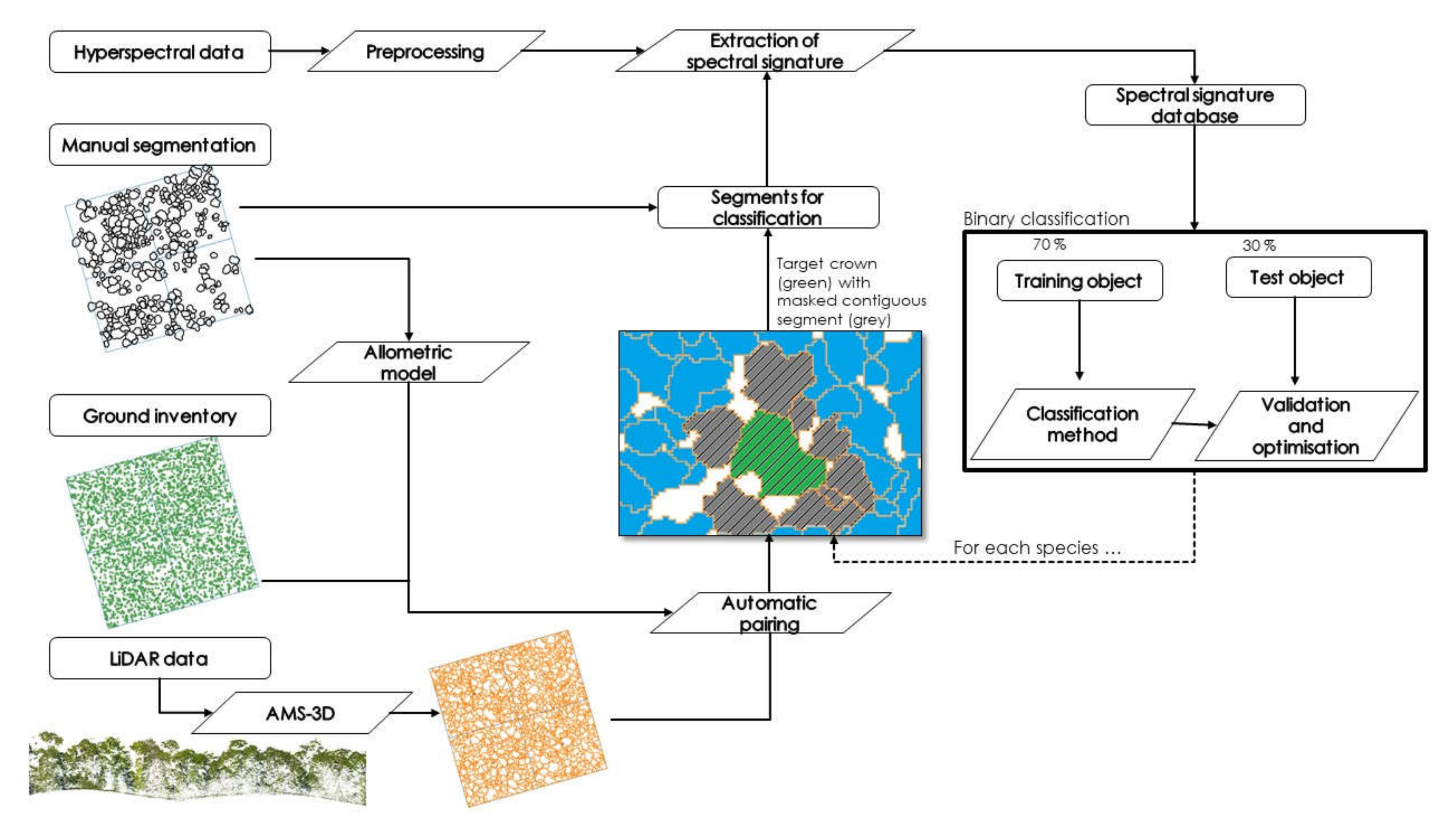
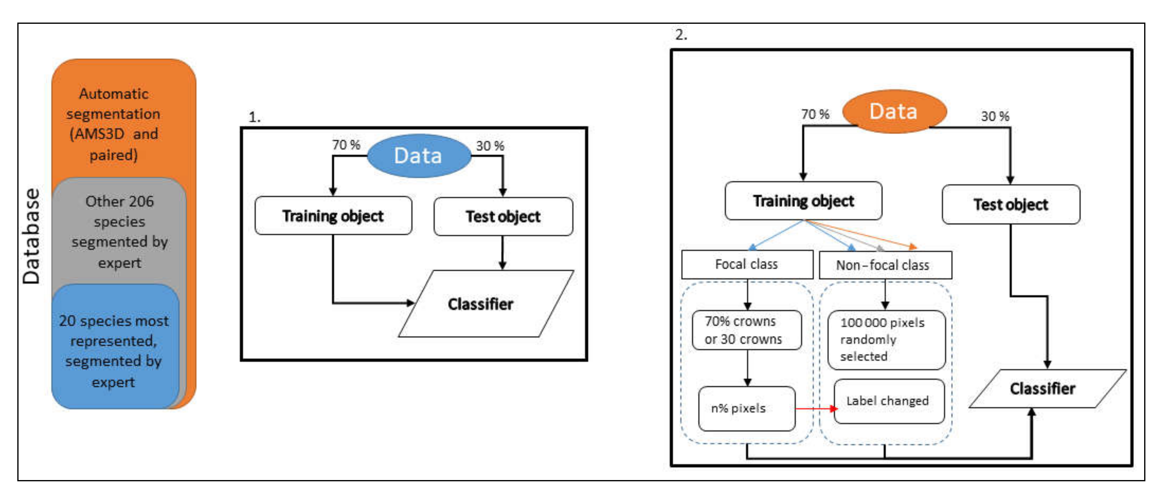
2.2. General Methodology Outline

The general methodology is outlined in Figure 1. LiDAR data was used to segment crowns (Section 2.4.1) over the entire area of interest (118.75 ha). Manual segmentation (Section 2.3.3) and ground referencing was used to build a reference spectral signature database and species-specific allometric models. Inventory data (Section 2.4.2) were then paired with the automatically segmented (Section 2.4.1) crowns based on size and geolocation congruence.

The spectral signature database was used to train the binary classifiers, developed for each focal species (Section 2.5). The automatically delineated and labeled segments were used to mask the focal species across the whole area of the permanent plots to ensure a high level of purity of the non-focal class. To ensure that the non-focal class contained as few pixels as possible from the focal class, we considered a buffer around the crowns determined by the automatic assignment as belonging to the focal class. All contiguous segments and the segment itself were excluded from the training and testing sets (Figure 1).

2.3. Remote Sensing Data

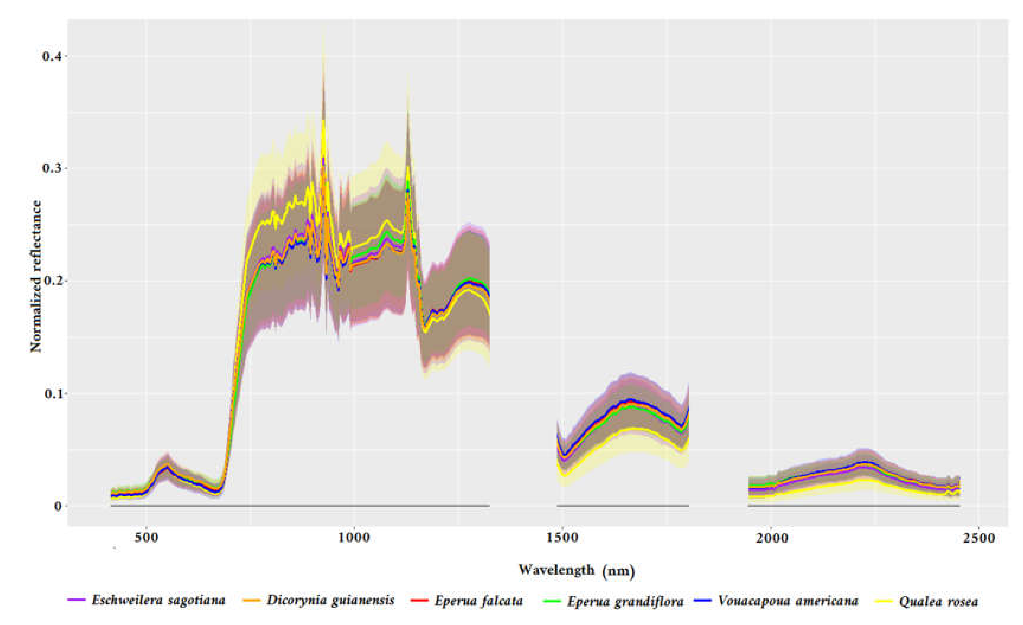
2.3.1. Hyperspectral Imaging

Imaging spectroscopy data was acquired with a Hyspex VNIR-1600 and a Hyspex SWIR-384 (Hyspex NEO, Skedsmokorset, Norway) sensor. The VNIR-1600 sensor covers the range from 414 nm to 1000 nm with 160 spectral bands and a spectral sampling distance of 3.64 nm. The SWIR-384 sensor covers the range from 1000 nm to 2500 nm with 288 spectral bands and a spectral sampling distance of 5.45 nm. The entire spectral range of the VNIR sensor was used. The information acquired in the SWIR domain is sensitive to atmospheric water absorption, so the spectral information corresponding to the low signal-to-noise ratio domains was discarded. Finally, the following spectral windows were kept: for the SWIR domain: 1009 nm to 1318 nm, 1454 nm to 1796 nm and 1964 nm to 2458 nm. Hence, 195 SWIR bands were retained. The King Air B200 airplane flew at an average altitude of 920 m. The flight took place on a cloudless day (from 15:00 to 17:00, solar time) on the 19th September 2016. Images were orthorectified and georeferenced with the PARGE software [31] using the canopy DSM (digital surface model) produced from the LiDAR point cloud (see next section). The DSM was created from the point cloud by selecting point of maximum height on a 1-m resolution grid. The spatial resolutions of the VNIR and SWIR images were 1 m and 2 m respectively. In order to merge the data without degrading the spatial resolution of the VNIR imagery, we resampled the SWIR imagery at 1 m using the nearest neighbor method. In addition, the fields of view of the two sensors are not identical (17° and 16°). We constrained the spectral information to the narrowest field of view corresponding to the one of the SWIR sensor. In the end, we obtained VSWIR imagery covering the entire spectrum (414 nm to 1963 nm) corresponding to 355 bands. Spectral information used to train the species classifiers was extracted from flight lines rather than from a mosaic, as it was previously shown to be more effective [22]. Although the training was carried out on the flight lines, the prediction was done on the mosaic where the pixels with viewing angle closest to vertical were kept (“center cropped” option of PARGE software [32]).

Atmospheric correction was applied using ATCOR-4 software [31]. The water vapor was retrieved using the APDA (atmospheric pre-corrected differential absorption) algorithm. The aerosol optical thickness (AOT) represents the amount of aerosols in the entire column of the atmosphere. It was considered constant. Non-vegetated pixels were identified based on NDVI (normalized difference vegetation index) thresholding, following recommendations for wavelength selection given in [33].

$$NDVI=\frac{{\lambda }_{774}-{\lambda }_{676}}{{\lambda }_{774}+{\lambda }_{676}}$$

(1)

Pixels with NDVI values higher than 0.4 were considered vegetation. Then, we applied a spatial mean filtering and a spectrum normalization by the mean as described in [22]. The illumination ratio was used to remove pixels with a scaled shadow fraction value higher than 0.6.

2.3.2. LiDAR Data and RGB Imagery

Airborne laser scanning data and RGB imagery were acquired during the same flight as the hyperspectral data. The LiDAR system was an LMS Q780 RIEGL operated with the following characteristics: a scan frequency of 400 kHz, a scan angle of +/− 30°. Neighbouring strips overlapped by 90%. Final mean pulse density was 33 pulses·m⁻². In addition, RGB (red, green, blue) imagery was acquired during the same flight using an iXu 180 Phase One camera. The final spatial resolution of the RGB orthorectified mosaic was 10 cm.

2.3.3. Ground Reference Data

A field survey was conducted to build a large ground reference dataset distributed over 56 of the 76 plots monitored on the study site (87.5 ha). Easily discernible crowns were first delineated manually based on the canopy height model (CHM), derived from LiDAR data with the help of the high-resolution RGB mosaic. The correct delineation of these ITCs was then validated in the field and the corresponding species ascertained. The 20 most abundant species in the delineated ITC dataset represented 1297 ITCs with a minimum of 24 individuals per species. Another 949 crowns were delineated, corresponding to 226 species. In total, the labeled database contained 2246 trees (

Table 1. List of target species, and corresponding number of crowns and total number of pixels retained for analysis (each crown was imaged twice, but some pixels were removed due to low illumination or NDVI values). Sample representation refers to the proportion of manually segmented crowns of a given species. Mean crown area followed by standard deviation in brackets. Commercial species are underlined.

Species (Acronyms)	Number of Crowns	Number of Pixels	Mean Crown Area (m2) (SD)	Sample Representation (%)
Qualea rosea (Q.r.)	206	27,828	109.5 (59.4)	9.2
Pradosia cochlearia (P.c.)	164	38,349	142.3 (122.5)	7.3
Eschweilera sagotiana (E.s.)	139	12,559	49.1 (29.0)	6.2
Dicorynia guianensis (D.g.)	108	18,589	102.7 (66.8)	4.8
Eperua falcata (E.f.)	106	15,355	71.7 (41.3)	4.7
Eperua grandiflora (E.g.)	74	10,859	87.3 (46.2)	3.3
Recordoxylon speciosum (R.s.)	69	7944	69.6 (26.2)	3.1
Tachigali melinonii (T.m.)	51	6745	106.2 (67.1)	2.3
Couratari multiflora (C.m.)	49	4850	55.1 (33.8)	2.2
Licania alba (L.a.)	46	3894	47.0 (18.4)	2.0
Symphonia sp.1 (S.s.)	34	3355	50.2 (20.1)	1.5
Vouacapoua americana (V.a.)	34	3218	65.4 (34.0)	1.5
Sextonia rubra (S.r.)	32	4070	118.5 (99.3)	1.4
Tapura capitulifera (T.c.)	32	1224	30.5 (12.2)	1.4
Licania heteromorpha (L.h.)	27	1437	40.3 (21.7)	1.2
Moronobea coccinea (M.c.)	27	3355	68.8 (36.7)	1.2
Inga alba (I.a.)	26	3846	81.3 (58.7)	1.2
Goupia glabra (G.g.)	25	4998	133.7 (77.3)	1.1
Bocoa prouacensis (B.p.)	24	2375	54.9 (35.8)	1.1
Jacaranda copaia (J.c.)	24	1705	40.4 (22.7)	1.1
Others	949	84,713	80.8 (71.6)	42.3

). Most crowns were imaged twice by hyperspectral sensors because of the overlapping flight lines. The normalized mean spectra and its standard deviation for the most abundant tree species is illustrated in Figure 2.

In the 20 plots where no manual segmentation of ITC was done, 532 species were recorded for a total of 19,379 trees.

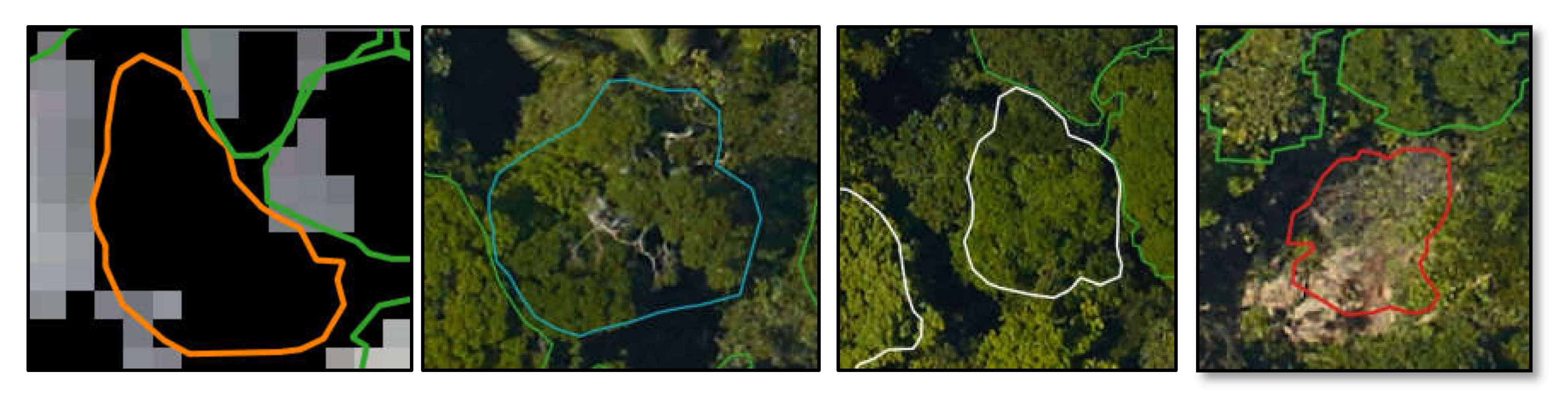
2.4. Automatic Segmentation Method

2.4.1. AMS-3D Method

We applied AMS-3D [34] to the LiDAR data for ITCs segmentation. The AMS-3D algorithm considers the point cloud as a multi-modal 3D distribution where each mode corresponds to the location of a tree crown. To find the modes, a Pollock function was used as bandwidth [35], with parameters changing with points’ height to allow higher crowns to be bigger [34]. Points converging to the same mode were attributed the same ITC. The 3D clusters corresponding to each crown were then projected vertically to obtain polygons. The point cloud segmentation was conducted with the Computree platform (http://computree.onf.fr/), and the projection with the R package lidR [36].

2.4.2. Correspondence between ITC and Inventory Data

The automatically segmented crowns were then paired with the inventory data, using a pairing algorithm based on allometric relation and distance between the crown and the stem [27]. First, using data from the manually segmented crowns, we modelled each tree DBH as a function of crown diameter, height and taxon:

$$ln\left(DB{H}_i\right)={\alpha }_{s{p}_i}+{\beta }_{s{p}_i}ln\left(H_i\times C{D}_i\right)+\epsilon$$

(2)

$$\epsilon \sim \mathcal{N}\left(0, {\sigma }_i^2\right)$$

(3)

where $DB{H}_i$ is the DBH (cm) of tree $i$ of species $s{p}_i$, $H_i$ is its height, $C{D}_i$ its crown diameter, and $\epsilon$ the error term. We then computed the distance between each manual segmented crown and all trunks of the inventory, computed the distance ranking of the trunk associated with the crowns, and fitted an exponential distribution on the ranks:

$$d_{i,j}=\alpha e^{-\alpha r_{i,j}}$$

(4)

where r_i,j is the rank of tree j associated with crown $i$, and α is the parameter of the exponential distribution. Then, we developed an algorithm to optimally pair a crown with a tree from the inventory using the model previously parameterized. This algorithm takes two types of information into account: (i) the distance between the crown center (computed as the 2D-centroid of crown projection) and the trunk location in the inventory should be close, and (ii) the tree should obey the allometric relation between the crown size and the trunk diameter. We considered those two rules to apply independently, neglecting a possible dependency of crown trunk distance on tree size. The pairing algorithm pairs each crown with the tree with highest:

$$p_{i,j}=d_{i,j}·g_{i,j}$$

(5)

where $g_{i,j}$ is the density function of the allometric model. Stems were ordered by decreasing DBH, and they were paired one after another in that order, with the segmented crown having the largest $d_{i,j}$ in the neighbourhood of the stem (15 m). When a crown was allocated to a stem, it was no longer available for others. Details of the algorithm can be found in [27].

2.5. Classification Method

We compared three classification methods for tree species identification: linear discriminant analysis (LDA), regularized discriminant analysis (RDA) and logistic regression (LR). We used the python language and the sklearn library [37]. The optimization of hyperparameters for the LR required considerable computing power. We used a Singularity container [38] and ran the code on a cluster of computers.

The LDA classification algorithm is well adapted to classification problems in high-dimension feature spaces provided that the number of observations is larger than the number of features in the least abundant class [39]. The principle of LDA consists in calculating new variables called discriminating canonical variables as linear combinations of the initial variables. It is calculated to maximize the ratio of the inter-group variance to the intra-group variance.

RDA is a compromise between LDA and quadratic discriminant analysis (QDA). QDA is a variant of LDA, the former being better adapted for non-linear separation. LDA assumes multivariate normal distribution of features with a common covariance matrix and different mean vector for each class. As shown by [40], LDA is not sensitive to the normal distribution assumption. Nevertheless, when the assumption of common covariance matrix is not satisfied, the individual covariance matrix for each group should preferably be estimated. This specific step characterizes QDA. The discriminating boundaries of the QDA are quadratic curves. The intermediate method between the two gives the RDA method proposed by [41] and makes it possible to regularize group covariance matrices, while preserving its performance in multi-dimensionality [42].

The assumptions of multivariate normality and equal variance–covariance matrices between groups are required before proceeding with LDA. On the contrary, in LR, these assumptions are not made. The authors of [43] showed in a bivariate case that in binary classification LR would be more efficient as soon as the normality assumption would be violated. A regularization term penalizing large values of the parameters was considered to avoid possible overfitting during the training step. A penalty parameter controlling the relative cost of errors occurring in the two classes was also tuned. We used a grid search to find the best combination of hyper-parameters C (regularization) and w_c (relative focal class weight) over the values C {e⁰, e¹, e²,…, e⁶ } and $w_c${1,2,…,10 }. In case of bias (impure non-focal class), we used the criterion of [29], otherwise we used the F-measure metric (see below).

2.5.1. Classifier Evaluation Criteria

To assess the reliability of the binary classifier, the F-measure was the chosen accuracy measurement. It relies on the estimation of the precision and recall of the class of interest. F-measure was used instead of accuracy due to the difference in proportion between the classes. The precision is the number of correct positive results divided by the number of all positive results returned by the classifier, and the recall is the number of correct positive results divided by the number of all relevant samples (all samples that should have been identified as positive).

$$\mathrm{F}-\mathrm{measure}=\frac{2\times \mathrm{precision}\times \mathrm{recall}}{\mathrm{precision}+\mathrm{recall}}$$

(6)

$$\mathrm{Precision}=\frac{\sum \mathrm{T}\mathrm{P}}{\sum (\mathrm{T}\mathrm{P}+\mathrm{F}\mathrm{P})}$$

(7)

$$\mathrm{Recall}=\frac{\sum \mathrm{T}\mathrm{P}}{\sum (\mathrm{T}\mathrm{P}+\mathrm{F}\mathrm{N})}$$

(8)

TP, FP and FN refer to true positive, false positive and false negative, respectively.

For comparison between LDA, RDA and LR, we used the exact same randomly sampled training and testing sets.

2.5.2. Optimization Step

All classifiers used in this study output a probability for a pixel of belonging to the focal class, which is defined by the maximum likelihood. The threshold used for assignment to the focal class can be refined by using a specified criterion, to improve the classification performance. We used different criteria for the standard (unbiased) case and when the non-focal class was impure. In the standard case, we sought to maximize the pixel level F-measure. When dealing with the mislabeled non-focal class (i.e., when the non-focal class contained pixels of the focal class), true precision was unknown, so we sought to maximize the following quantity [29]:

$$\frac{Recal{l}^2}{P\left(f\left(x\right)=1\right)}$$

(9)

where the $Recall$ is recall of the accuracy and P[f(x) = 1] is the probability that a sample is classified in the focal class.

2.6. Experimental Set-Up

We present four different experiments. All classifiers considered in this study were binary classifiers; i.e., a particular focal species is classified against a large set of non-focal species. As a rule, we separated the data into 70% of the crowns used for the training set and 30% for the test set (Figure 3) repeating the operation 30 times. We provide the mean and the standard deviation of the F-measure.

We first compared classification performances obtained when using spectral information from either VNIR or VSWIR on the 20 most abundant species only (Experiment 1). Then, we explored how the performance of the classifier would be affected by gradually increasing the number of species among which our focal species was retrieved (Experiment 2). In a third experiment, we explored the sensitivity of the classifiers to different types of errors affecting the training data (labeling errors) (Figure 3, Experiment 3). In a final test (Experiment 4), we predicted the basal area of focal species per 1.56 ha plot from the hyperspectral data.

2.6.1. Experiment 1—VNIR versus VNIR+ SWIR

We assessed the effectiveness of adding SWIR bands to the VNIR spectrum. We used manual segmentation data and we selected the 20 most abundant tree species (Figure 3, 1). The same pixels were used to build training and test sets (70%–30%) for VNIR and VSWIR data. For this first experiment, none of the three classification methods were subject to secondary optimization.

2.6.2. Experiment 2—Increasing Background Spectral Diversity

The same 20 focal species were considered for this experiment, but we gradually added more species to the non-focal class. We first added the crowns of the most abundant species present in the manually segmented crowns database, up to 99 different species. We then added all the remaining crowns from the manual segmentation database (each crown being the sole representative of its species) in arbitrary order. Thereby, the 364 different species were opposed to each of the 20 species alternately. For this first experiment, LDA was used, without an optimization step.

2.6.3. Experiment 3—Effect of Noise in the Training Data

In an operational case, the inventory effort will likely be focused on few target species. Thus, the other non-focal species will not be systematically inventoried. Therefore, to train the classifier, the non-focal species class will be represented by a random selection of pixels over the entire study area (excluding crowns known to belong to the focal species). However, the probability for a pixel of the focal class of being selected and contributing to the non-focal class is dependent on the distribution of this species in the study area, viewed at canopy level.

To assess the impact of a given level of mislabeling of the non-focal pixels, we artificially biased the learning data set (Figure 3, 2). We randomly selected 100,000 pixels from the background, excluding the focal species to create the training set for the non-focal species. We simulated three level of bias in the training data by successively replacing 1%, 2% and 5% of the pixels labeled as belonging to the non-focal class with pixels taken from crowns of the focal species class.

We also explored the potential impact of mislabeling of the focal pixels, reckoning that such errors may occur regardless of the efforts made in the field (identification errors, matching errors, etc.). We used Mahalanobis distance to detect outliers among the 20 most abundant species in the manually segmented crown database. For each species, we computed this multi-dimensional distance for each pixel, we then computed the mean Mahalanobis distance per crown. Crowns beyond two standard deviations were considered as pseudo-outliers and removed from the database. Binary classifications using all the information (including pseudo outliers) were then compared to those excluding pseudo-outliers.

Mahalanobis distance is a multi-dimensional distance measure between a point and a distribution. This distance d(x) can also be defined as a dissimilarity measure between a vector and a mean vector from the same distribution:

$$d\left(\overrightarrow{x}\right)=\sqrt{{\left(\overrightarrow{x}-\overrightarrow{u}\right)}^T{{\displaystyle \sum }}_{}^{-1}\left(\overrightarrow{x}-\overrightarrow{u}\right)}$$

(10)

where $x$ is a spectrum, $u$ the mean spectrum, Σ is the variance–covariance matrix.

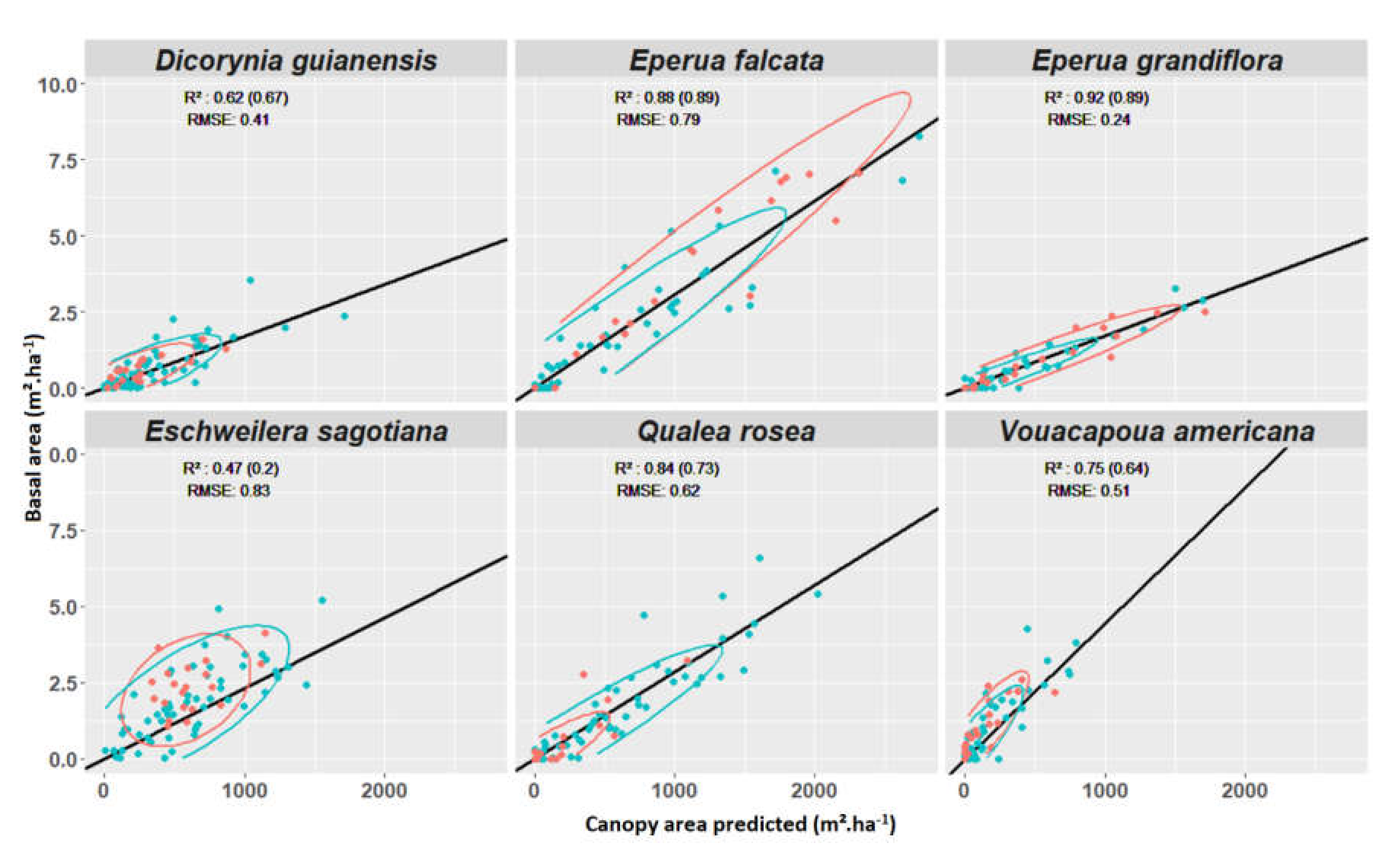
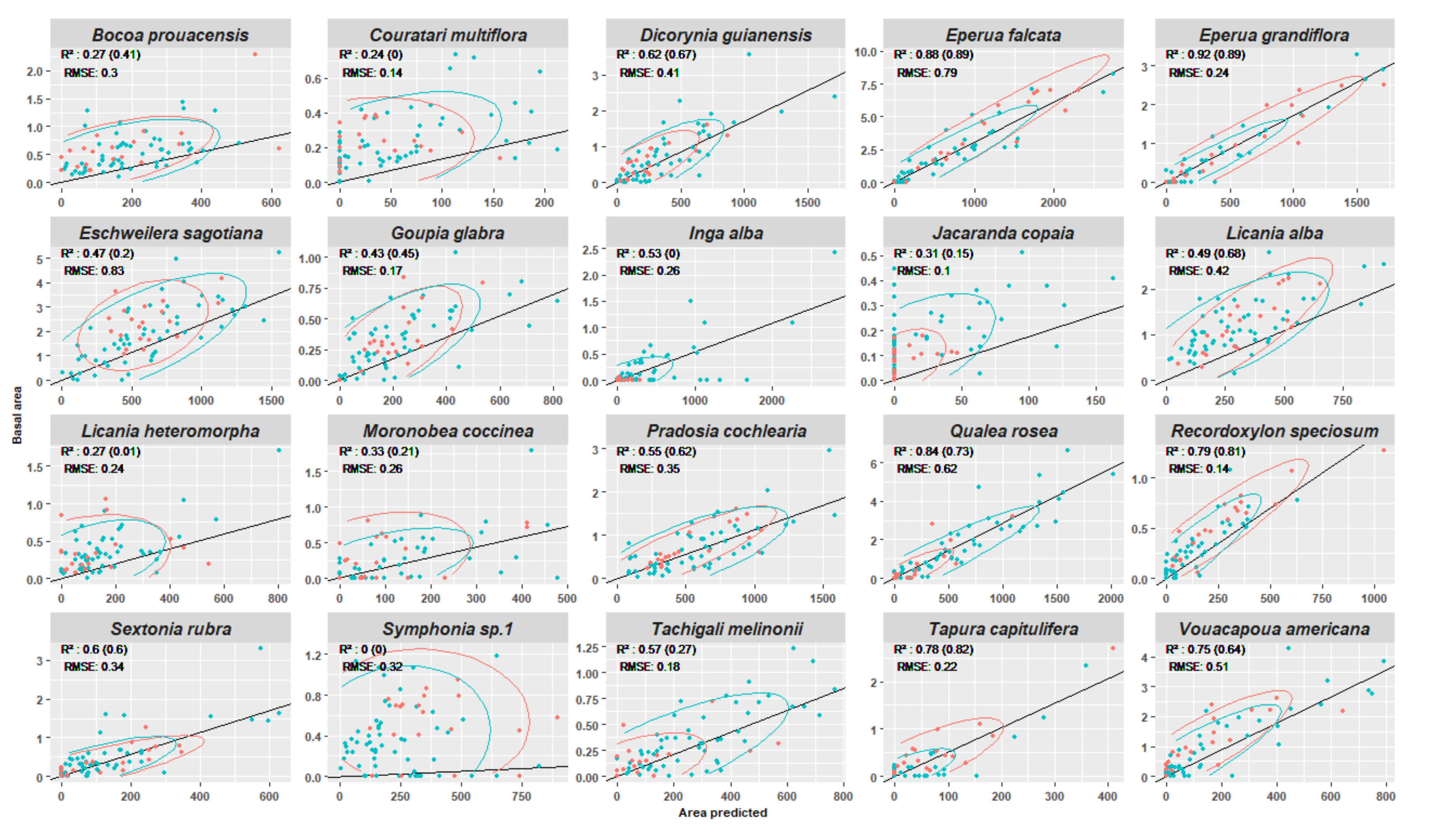
2.6.4. Experiment 4—Predicting Basal Area per Species per Plot

The ground inventory data comprised 76 plots of 1.56 hectares. For each plot, we compared the canopy surface predicted per species (at crown and pixel level) by the best-performing classification method and the basal area of the species using a linear regression. The learning step used all the information on the focal species which was available in the manually segmented crown database to build the focal class and 100,000 pixels randomly selected from the same 56 plots. Hence, 20 plots (c. 25% of the area) were set aside to be used for independent validation. The learning step used 100,000 pixels from flight lines, while the prediction was realized on the mosaic.

We compared prediction of the three classifiers applied with and without an optimization step and with or without majority vote at crown level. The majority vote rule was applied to decide on the species label to be assigned to ITCs, which corresponded to a filling rate higher than 50% of the pixels. We present the results obtained with the LDA only. The basal area considered here is the basal area of all trees with DBH greater than 10cm. It may be noted that smallest trees will not be visible in the areal imagery.

3. Results

3.1. Experiment 1

The combination of VNIR and SWIR information strongly improved the performances of all classifiers compared to VNIR information only, with an increase in F-measure of 23.8%, 27.3% and 19.4% for LDA, RDA and LR respectively. The contribution of SWIR was very important for all species. The difference between LDA and RDA was not significant in this case. All species were rather well identified (F-measure never lower than 59%). LR did not outperform LDA nor RDA.

Moderate differences in performance were observed between classifiers when only the VNIR information was used. LR performed slightly better than the other two methods except for Eschweilera sagotiana (70% vs. 79%) and RDA appeared to perform slightly worse, particularly at pixel level (Appendix A). The change from pixel to object level was confirmed to be very beneficial. LDA gained the most from the majority vote, with an increase of 15.5% in F-measure using the complete VSWIR information (

Table 2. Comparison of the F-measure at object level (and standard deviation) obtained after classification with the three methods when either VNIR or VSWIR information are used. Commercial species are underlined. The best prediction for each species with either VNIR or VSWIR information is in bold.

Species	VNIR			VSWIR
	LDA	RDA	LR	LDA	RDA	LR
B.p.	25.4 (±11.6)	22.3 (±8.5)	26.4 (±7.2)	66.9 (±11.3)	83.3 (±10.4)	61.0 (±18.0)
C.m.	66.7 (±13.2)	64.8 (±13.5)	67.5 (±11.0)	75.0 (±10.7)	67.9 (±9.9)	77.0 (±8.4)
D.g.	61.2 (±4.5)	61.3 (±4.7)	69.2 (±7.0)	88.6 (±2.5)	86.3 (±3.6)	90.3 (±2.4)
E.f.	46.9 (±5.5)	7.3 (±2.5)	29.6 (±9.6)	70.0 (±5.8)	72.9 (±8.2)	73.9 (±6.7)
E.g.	63.1 (±6.4)	61.8 (±7.4)	79.4 (±5.0)	82.1 (±5.3)	87.6 (±4.4)	89.7 (±3.6)
E.s.	79.0 (±3.3)	72.8 (±5.3)	70.6 (±7.3)	89.6 (±2.8)	89.3 (±1.9)	86.4 (±2.1)
G.g.	44.3 (±8.9)	63.3 (±12.1)	67.6 (±12.9)	84.1 (±7.3)	83.9 (±12.0)	80.4 (±12.7)
I.a.	44.4 (±14.2)	49.4 (±15.6)	62.7 (±17.2)	77.6 (±10.0)	76.3 (±8.5)	66.0 (±16.0)
J.c.	58.4 (±16.7)	59.2 (±12.6)	57.1 (±16.6)	59.2 (±19.1)	58.2 (±18.1)	70.2 (±16.8)
L.a.	55.9 (±10.0)	62.9 (±10.7)	62.6 (±11.4)	78.1 (±4.5)	79.6 (±9.5)	74.6 (±9.1)
L.h.	22.2 (±8.0)	16.7 (±0.0)	20.0 (±0.0)	65.2 (±11.3)	60.7 (±13.7)	49.0 (±14.6)
M.c.	64.5 (±11.4)	52.7 (±14.3)	64.1 (±13.3)	82.8 (±10.9)	74.7 (±17.4)	79.7 (±12.7)
P.c.	80.5 (±4.2)	83.6 (±3.8)	88.4 (±3.3)	93.5 (±1.9)	93.6 (±1.9)	94.1 (±1.6)
Q.r.	94.8 (±1.6)	94.6 (±1.5)	95.6 (±1.2)	96.9 (±1.1)	96.2 (±1.4)	97.2 (±1.1)
R.s.	84.9 (±6.0)	81.4 (±5.0)	90.0 (±4.7)	91.4 (±3.3)	87.1 (±6.1)	90.6 (±3.8)
S.r.	55.0 (±9.2)	50.6 (±14.5)	53.7 (±13.2)	77.6 (±11.5)	82.9 (±8.4)	85.2 (±7.3)
S.s.	24.0 (±0.0)	0.0 (±0.0)	11.3 (±0.0)	64.0 (±11.7)	68.9 (±12.1)	50.5 (±13.7)
T.m.	73.3 (±7.7)	79.2 (±6.0)	84.1 (±5.6)	93.5 (±4.1)	93.3 (±4.3)	93.4 (±4.1)
T.c.	35.4 (±8.7)	17.1 (±4.0)	38.2 (±14.1)	82.6 (±8.9)	72.7 (±11.8)	83.5 (±9.8)
V.a.	48.7 (±13.8)	52.8 (±13.7)	43.0 (±14.7)	85.1 (±8.3)	83.8 (±10.0)	77.1 (±10.1)
Mean F-measue	56.4	52.7	59.1	80.2	80.0	78.5

).

3.2. Experiment 2

We gradually added crowns from new species to increase the spectral variability of the non-focal class. We used an LDA binary classifier to retrieve each of the 20 most abundant species. No optimization was applied. We present the results at object level (following majority vote).

The overall trend in Figure 4 highlights that increasing the number of species degraded the classifier’s performance. Some species were highly affected (e.g., Eschweilera sagotiana); others were only slightly affected (e.g., Qualea rosea). Increasing the number of species from 99 to 364 significantly affected discrimination of all target species. F-measure for Qualea rosea, the best-identified species, decreased from 88.6% to 84.9%, a loss of about 4% points.

The F-measure value for the species Licania alba, Licania heteromorpha and Inga alba declined sharply with the added species. In these cases, the focal species was well retrieved (the recall was higher than 70%), but the precision was very low (a lot of pixels were wrongly predicted to belong to the focal class).

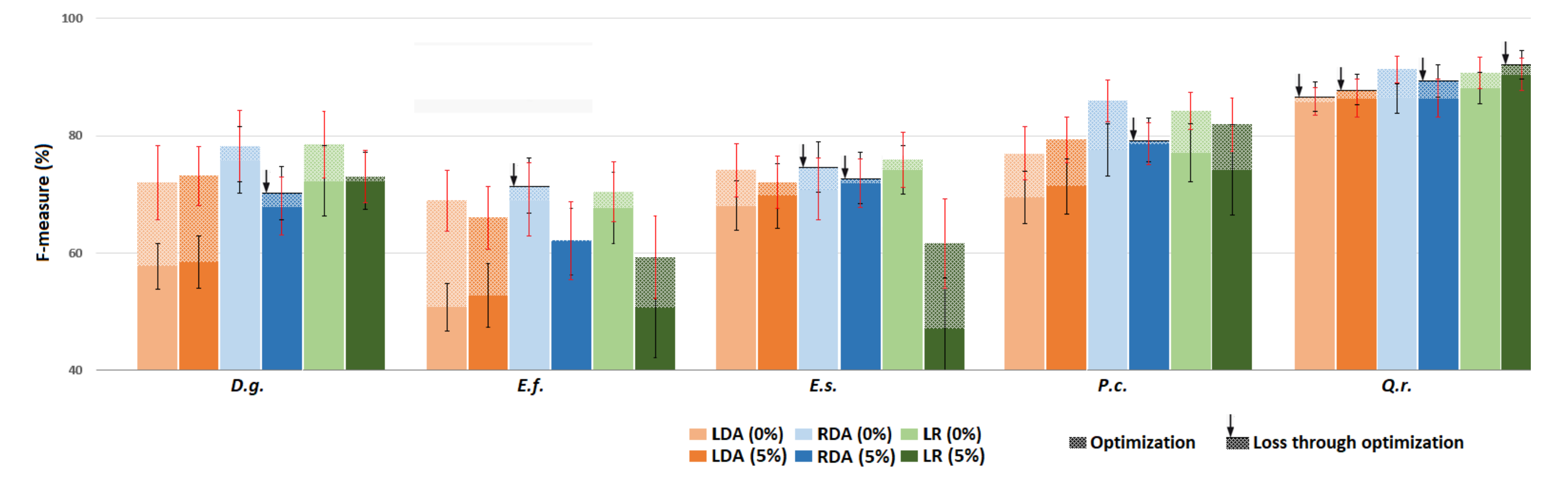
3.3. Experiment 3 –Exploring the Impact of Training Set Impurity

To evaluate the impact on the classification performance of mislabeled pixels in the non-focal class, we applied different levels of contamination bias (1%, 2% and 5%).

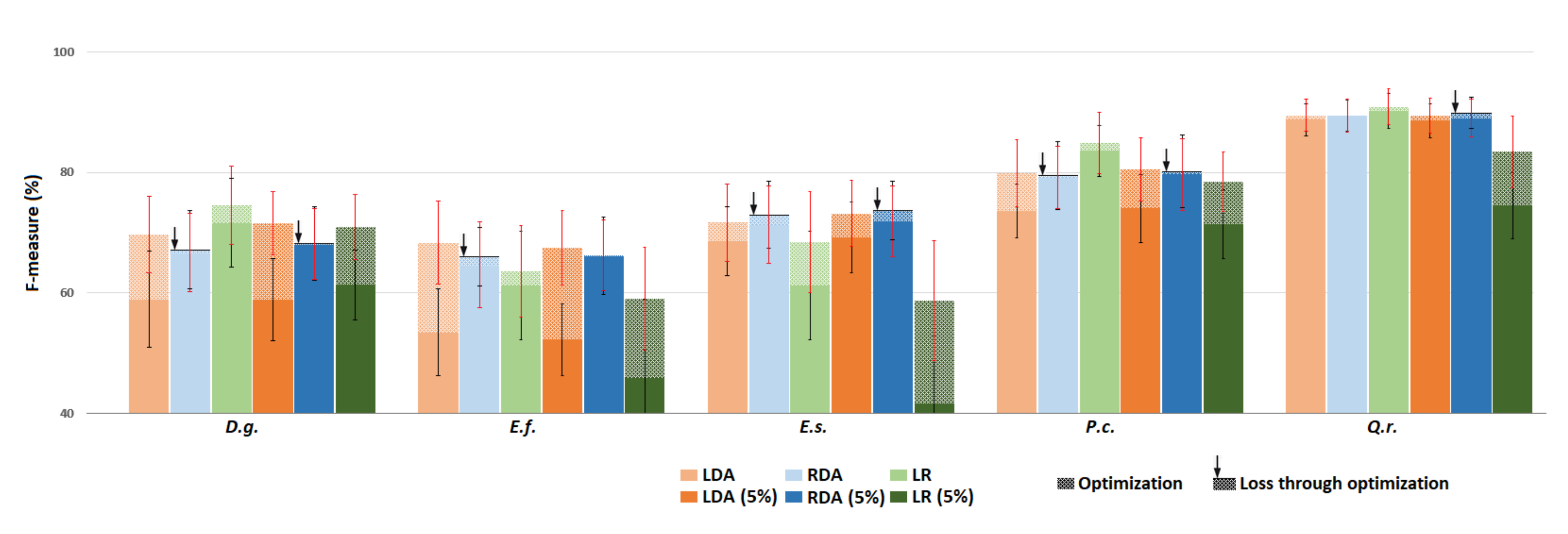
3.3.1. Low Level of Impurity (All Species)

We first examined to what degree the different classification methods were affected by a low level of impurity of the non-focal class, and whether optimizing the pixel threshold based on the criterion proposed by [29] could mitigate this bias.

A noise of 1% had no significant effect on the identification of species, whether an optimization step was used or not (

Table 3. Object level F-measure (and its standard deviation in brackets) of species binary classifiers trained with 1% mislabeling of the non-focal class. Plain and optimized indicate whether an optimization step (selecting a threshold probability value) was applied to maximize either the F-measure (0% contamination) or the Lee and Liu 2003 criterion (1% contamination). Standard deviation is given in Appendix B. The best prediction for each species and method is in bold.

Bias	0%						1%
	Plain			Optimized			Plain			Optimized
Species	LDA	RDA	LR	LDA	RDA	LR	LDA	RDA	LR	LDA	RDA	LR
B.p.	35.8 (±10.3)	57.7 (±12.4)	37.5 (±15.5)	65.4	57.5	42.1	36.4	58.5	43.4	64.3	56.2	43.0
C.m.	68.3 (±10.8)	64.7 (±10.1)	68.0 (±10.5)	69.8	68.3	71.4	67.4	65.1	66.5	69.8	68.0	69.4
D.g.	57.7 (±3.9)	72.3 (±6.0)	78.2 (±6.1)	75.8	72.0	78.5	57.5	72.6	78.2	74.8	72.2	78.3
E.f.	50.8 (±4.1)	67.7 (±6.1)	69.2 (±6.2)	71.5	68.9	70.5	51.5	67.9	68.0	72.1	69.2	70.5
E.g.	65.1 (±7.0)	82.0 (±5.3)	84.4 (±4.6)	82.4	82.7	84.8	64.9	81.9	82.5	82.0	82.5	84.7
E.s.	68.1 (±4.2)	74.2 (±4.1)	71.0 (±5.2)	74.7	74.1	75.9	68.5	74.7	69.2	74.1	73.4	74.9
G.g.	62.5 (±12.6)	73.4 (±11.5)	76.4 (±12.5)	74.5	73.5	77.3	62.8	72.6	74.8	74.5	74.4	75.0
I.a.	38.3 (±11.5)	42.3 (±12.7)	38.5 (±11.6)	43.0	41.0	41.4	38.9	42.7	36.6	43.0	41.4	40.9
J.c.	50.7 (±19.7)	51.4 (±16.8)	52.4 (±17.1)	50.9	49.3	53.1	52.2	49.0	51.6	51.5	50.4	52.6
L.a.	41.6 (±8.7)	56.3 (±10.8)	53.9 (±10.5)	56.6	54.4	62.3	41.9	56.8	48.5	57.0	54.7	59.7
L.h.	25.6 (±8.9)	43.6 (±11.0)	22.8 (±8.1)	44.0	34.2	25.5	26.5	43.5	23.5	46.6	33.7	26.0
M.c.	58.5 (±13.8)	55.5 (±16.9)	60.0 (±14.5)	56.3	54.9	62.7	58.6	56.1	56.5	55.4	56.2	61.7
P.c.	69.5 (±4.5)	77.1 (±4.9)	85.9 (±3.6)	77.6	77.0	84.3	69.6	78.0	85.8	78.2	77.4	84.0
Q.r.	86.6 (±2.5)	88.1 (±2.7)	91.3 (±2.3)	86.4	85.8	90.7	86.9	88.1	91.2	86.6	86.2	90.8
R.s.	82.5 (±3.8)	78.8 (±4.5)	81.2 (±5.2)	81.0	80.7	84.9	82.4	79.3	79.5	80.7	79.7	83.4
S.r.	54.3 (±9.2)	70.8 (±10.7)	61.6 (±14.7)	71.8	66.9	68.0	53.8	69.7	52.3	71.3	66.4	61.1
S.s.	29.1 (±5.9)	36.7 (±9.1)	21.3 (±7.1)	36.6	36.7	25.6	29.1	35.8	21.3	35.5	35.8	25.6
T.m.	64.7 (±6.4)	69.9 (±6.0)	80.7 (±9.4)	76.3	75.8	78.8	64.9	70.4	78.2	76.0	75.6	78.9
T.c.	58.3 (±11.5)	65.4 (±12.5)	72.2 (±14.8)	65.8	52.1	72.5	58.2	65.4	69.6	63.6	51.0	70.6
V.a.	68.2 (±8.7)	72.8 (±12.2)	65.1 (±12.8)	74.4	74.4	66.9	66.5	74.1	63.9	74.4	73.6	64.6
Average	56.8	65.0	63.6	66.7	64.0	65.9	56.9	65.1	62.0	66.6	63.9	64.8

). When no optimisation was applied, LDA was outperformed by the other two methods for most of the species. For some species, LR was more efficient (e.g., Pradosia cochlearia) while for other species (e.g., Sextonia rubra) RDA performed best. Once optimized, all methods performed on a par in this experiment.

3.3.2. High Level of Impurity (Most Abundant Species)

This analysis was restricted to the five most abundant species in order to explore the effect of high rates of contamination of the non-focal species, which required having sufficient focal pixels. Results are summarized in Figure 5.

A labeling error of 5% did not affect LDA, with or without an optimization step. However, the optimization step was very beneficial in both cases. RDA was mildly affected by labeling error and not improved by optimization. LR classification method was much more impacted by a 5% error level and the optimization only partially compensated for this. The average loss in F-measure was 11.8% (without optimization) and 6.7% (with optimization). More complete results on the average F-measure, with or without an optimization step are provided in Appendix B, including results obtained for 2% bias.

In summary, RDA appeared to be robust to high noise level even without optimization. LR was sensitive to noise even after including a modified optimization step criterion [29]. LDA performed very well, provided that an optimization step was included.

3.3.3. High Level of Impurity—Smaller Focal Training Class

To assess the impact of the size of the focal class on classification performance we reduced the number of crowns to 30 in the focal class while still considering 100,000 pixels randomly selected for the non-focal class. Only the five most abundant species were considered. Miss-labeled pixels were added to the non-focal class to achieve different levels of contamination (1%, 2% and 5%). Results were almost undistinguishable from those obtained with larger training sets for the same level of bias (see Appendix C).

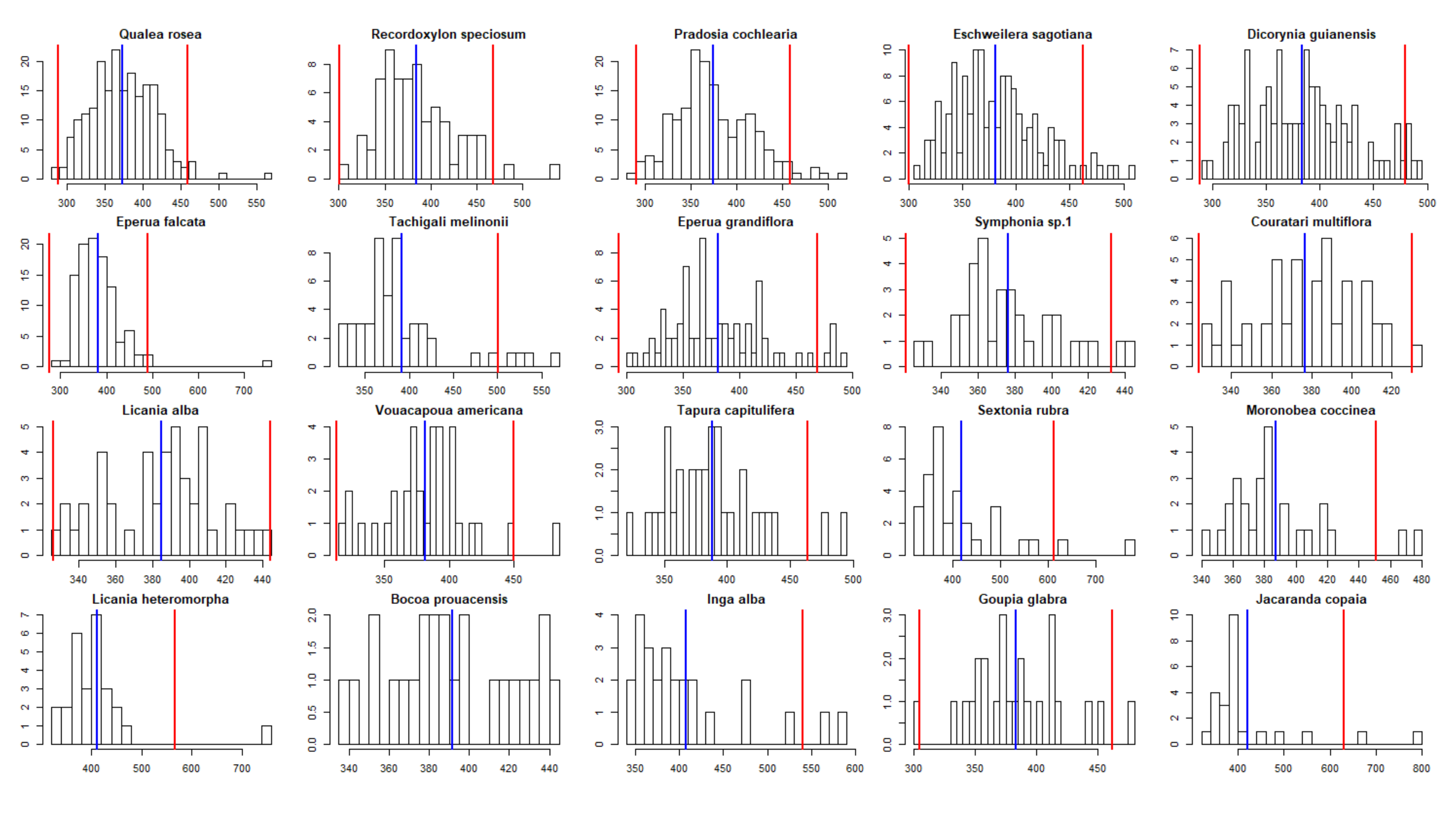
3.3.4. Focal Class Purification

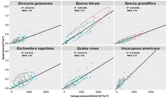
Mean crown Mahalanobis distance (computed across pixels within species) was used to try to detect outliers (Figure 6). Only Licania alba and Bocoa prouacensis had no outliers (outliers being defined as crowns showing a mean Mahalanobis distance greater than two standard deviations from the mean of all crowns). The most heavily impacted species were Jacaranda copaia and Goupia glabra (see table in Appendix D). Overall, for the 1297 representatives in the 20 focal classes, 55 crowns were potential outliers. There was thus a global potential bias of the focal classes of 4.2% or 2844 unreliable spectra.

We examined all those potential outliers on high-resolution RGB imagery. In a few cases, those outliers could be related to particular features (illustrated in Appendix D): low illumination leaving very few pixels per crown after filtering, higher than average contribution of wood caused by partial leaflessness (especially for Eperua falcata), presence of liana in the crown. However, in 90% of the cases, no peculiarity was detected on high-resolution imagery. One cannot exclude that crown mislabeling occurred, but this could not be ascertained.

To evaluate the improvement achieved after removing potential outlier crowns, a Student test by species was performed on each metric at object level for the three classifiers (without the optimization step). We compared those metrics before and after removal of the potential outliers. The most impacted species were the Couratari multiflora (from 68% to 71.6% using LR) and Sextonia rubra (from 61.6% from 64.7% using LR) (p-value <0.01). Recordoxylon speciosum (from 81.2% to 83.8% using LR) and Jacaranda copaia (from 50.7% to 59.2% using LDA) were less impacted (p-value <0.05). The RDA method was the method least sensitive to the introduction of outliers. For more detail, see the table in Appendix D.

3.4. Experiment 4

We related the recorded basal area per species per plot with the canopy area predicted to belong to the same species by the different classifiers. We used all the available crowns in our manual segments database to train the classifiers. For each focal species, we randomly selected 100,000 pixels to create the non-focal class for training the classifier. Results for LDA are reported in Figure 7 for the most abundant commercial species. Results for all other species are provided in Appendix E, Figure A3.

As expected, the effectiveness of the classifier conditions the correlation between the predicted canopy area and the basal area. The mean linear correlation coefficient across species was 0.70 (n = 20; Appendix F). Optimized LDA and RDA were the methods that provided the best average R² both at pixel and object level (not shown).

In addition, we compared the slope of the relations across species. We used a linear model without intercept. While species effect was significant overall (p < 0.01, e.g., Eperua grandiflora vs. Eperua falcata), some species shared a very similar slope (e.g., Qualea rosea vs. Vouacapoua americana). It might therefore be possible to use a common model between these species

Object-based prediction was better correlated to basal area than pixel-based prediction (4–8 point gain in R²) for all classifiers. Less than 2% of the pixels were classified into more than one species for both LDA and RDA. Hence, the confusion was low, despite the fact that the species-specific classifiers were developed independently. After majority voting, no confusion remained.

4. Discussion

The first experiment unambiguously confirmed that addition of SWIR information vastly improves classification performance. Our results on the contribution of SWIR information to species identification are in line with those obtained in previous studies [23,26,44]. The authors of [23] found that the LDA classification accuracy of seven tropical forest tree species was improved from 67.3% to 83.6%. Similarly, we found an increase in accuracy of about 20%–25% on average across species depending on the method considered. We noted that the gain was more important for LDA and RDA than for LR. In addition, we assessed the quality of our database. In fact, our database may contain a few mislabeled cases, as suggested by the Mahalanobis distance analysis. However, these outliers had a limited negative effect on classification in general. It is unclear how many of these pseudo-outliers are actual outliers. Phenology or presence of lianas was not found to be significantly associated with potential outliers.

The comparison of the results obtained in this study (Table 3, without bias) with previously published results (Table 4 in Laybros et al., 2019) indicates that there is no significant difference in performance between the binary and multiclass LDA classifier at pixel level. However, at the object level, the binary classifiers are clearly outperformed, implying a strong influence of the majority vote. The relative majority can be effective in a multi-class problem, whereas the absolute majority is required when only two classes are considered.

An important characteristic of our study case is the unbalanced number of spectra (pixels) in each class. The minority classes are the most affected by this constraint. Unbalanced classes impact results obtained with SVM classifications [45]. In some studies, the authors used SVM without a specific method to control for this effect [20,21,24,26,46]. This method is, however, sensitive to unbalanced classes [47,48,49,50]. Biasing the classifier by adding weights and breaking down the penalization of the classifiers (parameter C) into two parameters was recommended by [19,51] in order to reduce the negative impact of the minority classes. Conversely, LDA is not sensitive to the number of elements per class [52] because it shares the variance–covariation matrix between the classes. In addition, training on the entire data set or a subset of only 30 crowns did not affect the performance of the classifier. The similar results between the LDA and the RDA methods seem to confirm that RDA IS not sensitive to the disproportion between classes either.

It is preferable to optimize a specific metric in the biased cases and especially with a high bias rate. F-measure is not a good choice, because the precision is biased to an unknown extent. The use of the criterion proposed by [29] proved useful. In addition, when the bias is very severe, it is recommended to use a threshold that will optimize discrimination [49]. In the present study, LR was found to benefit much from this methodology. Conversely, the optimal probability threshold did not improve species discrimination for RDA.

The maximum level of bias tested here was 5%. How likely are larger biases to occur? In an operational case, the random selection of pixels on the study area will comprise a range of species reflecting the local flora of the study site. Despite the extremely high local tree species diversity (alpha diversity) in tropical forests [53], some species are spatially aggregated as a result of either environmental preference or dispersal limitation. For example, the Eperua falcata measured in the Piste de St Ellie region, is a species with an aggregated spatial distribution [54]. Vouacapoua americana, Eperua grandiflora and Qualea rosea species were also reported as being highly aggregated [55,56]. Extreme cases of aggregation may lead to monodominance [57], where more than 50% of the stems belong to a single species (e.g., Spirotropis longifolia). This, however, is a rare case and local frequency of the focal species will seldom reach 5% [58].

Most previous studies focused on discriminating a few well-known species against each other, which is of little relevance to an operational context. Here, we focused on assessing the potential of classification methods using hyperspectral information for retrieving particular species in a diverse canopy. This problem was previously addressed by [19], who highlighted the feasibility of identifying four tree species in a tropical forest canopy using biased SVM on the BCI site. As reported by [59], the taxonomic diversity in BCI is lower than in Paracou, whatever the diversity considered (alpha, beta or gamma diversity). On the BCI site, 225 tree species have been counted among more than 21,457 stems for an area of 50 hectares. On the Paracou site, 229 tree species were listed among 1124 stems for an area of 2 hectares. Therefore, the identification of focal tree species may be more challenging in the context of the present study than in the [19] study. As shown in Experiment 1, the performance of the classifiers tends to decrease with increasing diversity of the background.

The size of the training data set can be critical in an operational setting. The minimum number of crowns to be used for training in tropical canopies was investigated by [18,45]. Thirty crowns were found to be reasonable for species retrieval against 100,000 pixels. In the present study reducing the number of focal crowns from 74-144 to 30 crowns did not entail any loss in F-measure (comparison between Table 3 and Figure A1). However, the minimum training set size may depend on the species [18] and the diversity of the canopy. For the same number of crowns in the learning set (34 crowns, Table 1), the F-measure for Vouacapoua americana reached of 72.8% while it was only 36.7% for Symphonia sp.1 (Table 3, RDA). In addition, because classification results were so variable across species (Figure 4), we examined correlations between the predictability of the species (F-measure), the size of the focal species training set, the intra-specific spectral variance—sensu [60]—and the dispersion of the Mahalanobis distance values. The only significant correlation detected was with the size of the training set (number of crowns or number pixels) highlighting that the detectability of a species is difficult to predict (Appendix F,

Table A5. F-measure and various metrics tested for correlation.

Species	F-Measure (Object Level)	BA~CA r2	Number of Pixels	Number of Crowns	Intra Group Variance	Mean Species Mahalanobis Distance	Pseudo Outlier (%)
B.p.	65.4	0.27	2375	24	60716044	398	0
C.m.	69.8	0.24	4850	49	42710171	382	2
D.g.	75.8	0.62	18,589	108	88937469	383	4.6
E.f.	71.5	0.84	15,355	106	41768295	383	1.9
E.g.	82.4	0.92	10,859	74	37064303	378	6.8
E.s.	74.7	0.47	12,559	139	42879098	382	5
G.g.	74.5	0.43	4998	25	45436876	387	8
I.a.	43.0	0.53	3846	26	73845080	394	7.7
J.c.	50.9	0.31	1705	24	50504397	417	8.3
L.a.	56.6	0.49	3894	46	49323222	386	0
L.h.	44.0	0.27	1437	27	35529833	412	3.7
M.c.	56.3	0.33	3355	27	53471810	381	7.4
P.c.	77.6	0.55	38,349	164	46398429	374	3.7
Q.r.	86.4	0.84	27,828	206	51460549	374	3.4
R.s.	81.0	0.79	7944	69	120765823	382	2.9
S.r.	71.8	0.60	4070	32	31609536	417	6.3
S.s.	36.6	0.00	3355	34	38010280	378	5.9
T.m.	76.3	0.57	6745	51	80924196	392	7.8
T.c.	65.8	0.78	1224	32	36278962	388	6.3
V.a.	74.4	0.75	3218	34	137806130	387	2.9
Pearson Cor. Coeff	--	0.71 **	0.54 *	0.59 ***	0.28	0.08	0.48
Spearman Cor. Coeff.	--	0.69 **	0.77 **	0.71 ***	0.22	−0.44	−0.09

).

Forest managers need to quantify the resource of the forest in order to orient the choices to be made. We found the relation between basal area and crown area in the canopy to vary across species. The authors of [61] mention that a global allometric model can predict the diameter of the crown from the diameter of the stem. These estimates are based on more than 108,753 stems with different geographic locations, consisting of 1,492 tree species. However, this general relation is only valid at coarse grain, and studies comparing species occurring in a restricted geographical range repeatedly found marked inter-species differences. This was the case for Indian monsoon forest [62] and Sumatran peneplains agroforests [63], for instance. In addition, it should be stressed that, albeit visible from above (and therefore segmented and labeled), a crown may be partially masked by its neighbors, so the area of the visible segment can differ from the total crown area. Finally, errors stemming from the automatic segmentation step may have further blurred the basal area–crown area relation.

The use of LiDAR data allowed us to cluster points into putative crowns using the AMS-3D algorithm. This segmentation step allowed improving the performance of classifications through majority voting by an average of 10%–18%. This suggests that improving the segmentation step might provide improvement in the classification results. Segmentation itself may take advantage of multisource data. Depending of the way data are merged, fine co-registration can be required but may be difficult to achieve [64,65].

The next major challenge to address in remote species classification is transferring the knowledge acquired on one site to another one [22]. The spectral signature may vary over both space and time. One reason is variation in the timing of leafing, fruiting and flowering, which is still not well characterized for the vast majority of species in evergreen forest [66]. Tropical rainforest trees produce leaves with widely variable phenology and longevity [67,68]. Leaf optical properties may differ significantly between young newly sprouted leaves and one- to two-month-old fully mature photo-synthetically competent leaves [69]. In French Guiana where our study took place, a seminal work [70] monitored the phenology of 750 trees belonging to 35 species during two years. Various leafing patterns were reported to occur in that study: deciduous with synchronous or asynchronous leaf drop, or evergreen with continuous or seasonal leaf flushing. Local conditions (and notably soil water holding capacity) will contribute to desynchronize the phenological stage of deciduous trees submitted to similar weather conditions. Difference in tree water status may also alter leaf inclination through wilting which may affect the crown reflectance properties [71]. Additionally, differences in soil chemical fertility may induce differences in the spectral signatures of species. A long-known effect of an increase in nitrogen availability is an increased chlorophyll content and greenness [72]. The second major reason, and probably the most stringent issue, is the variability in imaging conditions. Several factors come into play to modify the apparent reflectance. On the one hand, during the acquisition, the sun–sensor angles change, as both the positions of the sun and the sensor are changing. The reflectance depends on those angles, and this dependency is idiosyncratic (i.e., depends on the characteristics of the object being imaged). Modelling the bidirectional reflectance distribution function (BDRF) to correct these spurious variations in spectral signature is extremely delicate. BRDF is likely to vary from tree to tree as it depends on characteristics such as foliage density, crown geometry (leaf size, leaf angle). Empirical or semi-empirical kernel-driven models [73] would probably require very large datasets to achieve a reasonable level of accuracy. The fact that reflectance in NIR is also significantly affected by neighbors identity [69] renders the hyper-diverse tropical forest particularly challenging in this respect.

5. Conclusions

We present a method that leverages the fusion of LiDAR data for ITC mapping and hyperspectral imagery for species identification. This method allowed us to accurately predict basal area of commercial species in a highly diverse tropical forest. As both types of sensors are likely to become more and more common, we hope that the proposed method will promote sustainable management of tropical forest.

Addition of the SWIR domain (1000nm to 2500nm) to the more commonly used VNIR spectrum was very useful and is strongly recommended whenever possible. In this study, we have examined different scenarios that forest managers may encounter to map specific species in tropical forests, including limited training set and labeling errors affecting both the focal and non-focal classes. We have successfully tested various methods to circumvent labeling error issues. We recommend using robust discriminant analysis, which seems to be the method least sensitive to bias while also offering very good results in the absence of bias in the training data. In addition, we have found that sampling can be limited to a few individuals (30 crowns) without reducing the accuracy of the classifications. Certain species were poorly identified with all classification methods. No indicator based on spectral characteristics allowed upstream identification of what made it possible to carry out an efficient classification of a given tree species.

References

1. Corlett, R.T. Plant diversity in a changing world: Status, trends, and conservation needs. Plant Divers. 2016, 38, 10–16. [Google Scholar] [CrossRef] [Green Version]
2. Peres, C.A.; Gardner, T.A.; Barlow, J.; Zuanon, J.; Michalski, F.; Lees, A.C.; Vieira, I.C.G.; Moreira, F.M.S.; Feeley, K.J. Biodiversity conservation in human-modified Amazonian forest landscapes. Biol. Conserv. 2010, 143, 2314–2327. [Google Scholar] [CrossRef]
3. Leisher, C.; Touval, J.; Hess, S.M.; Boucher, T.M.; Reymondin, L. Land and Forest Degradation inside Protected Areas in Latin America. Diversity 2013, 5, 779–795. [Google Scholar] [CrossRef] [Green Version]
4. Sala, O.E. Global Biodiversity Scenarios for the Year 2100. Science 2000, 287, 1770–1774. [Google Scholar] [CrossRef] [PubMed]
5. Burivalova, Z.; Şekercioğlu, Ç.H.; Koh, L.P. Thresholds of Logging Intensity to Maintain Tropical Forest Biodiversity. Curr. Biol. 2014, 24, 1893–1898. [Google Scholar] [CrossRef] [PubMed]
6. Putz, F.E.; Zuidema, P.A.; Pinard, M.A.; Boot, R.G.A.; Sayer, J.A.; Sheil, D.; Sist, P.; Vanclay, J.K. Improved Tropical Forest Management for Carbon Retention. PLoS Biol. 2008, 6, e166. [Google Scholar] [CrossRef] [Green Version]
7. Sist, P.; Mazzei, L.; Blanc, L.; Rutishauser, E. Large trees as key elements of carbon storage and dynamics after selective logging in the Eastern Amazon. For. Ecol. Manag. 2014, 318, 103–109. [Google Scholar] [CrossRef]
8. Putz, F.E. Woody vines and forest management in Malaysia. Commonw. For. Rev. 1985, 64, 359–365. [Google Scholar]
9. The Biology of Vines; Putz, F.E.; Mooney, H.A. (Eds.) Cambridge University Press: Cambridge, UK; New York, NY, USA, 1991; ISBN 978-0-521-39250-1. [Google Scholar]
10. Ouédraogo, D.-Y.; Beina, D.; Picard, N.; Mortier, F.; Baya, F.; Gourlet-Fleury, S. Thinning after selective logging facilitates floristic composition recovery in a tropical rain forest of Central Africa. For. Ecol. Manag. 2011, 262, 2176–2186. [Google Scholar] [CrossRef]
11. Alroy, J. Effects of habitat disturbance on tropical forest biodiversity. Proc. Natl. Acad. Sci. USA 2017, 114, 6056. [Google Scholar] [CrossRef] [Green Version]
12. Kennard, D.K.; Gould, K.; Putz, F.E.; Fredericksen, T.S.; Morales, F. Effect of disturbance intensity on regeneration mechanisms in a tropical dry forest. For. Ecol. Manag. 2002, 162, 197–208. [Google Scholar] [CrossRef] [Green Version]
13. Chaudhary, A.; Burivalova, Z.; Koh, L.P.; Hellweg, S. Impact of Forest Management on Species Richness: Global Meta-Analysis and Economic Trade-Offs. Sci. Rep. 2016, 6, 23954. [Google Scholar] [CrossRef] [PubMed] [Green Version]
14. Huang, C.; Asner, G.P. Applications of Remote Sensing to Alien Invasive Plant Studies. Sensors 2009, 9, 4869–4889. [Google Scholar] [CrossRef] [PubMed] [Green Version]
15. Ustin, S.L.; DiPietro, D.; Olmstead, K.; Underwood, E.; Scheer, G.J. Hyperspectral remote sensing for invasive species detection and mapping. In Proceedings of the IEEE International Geoscience and Remote Sensing Symposium, Toronto, ON, Canada, 24–28 June 2002; Volume 3, pp. 1658–1660. [Google Scholar]
16. Waite, C.E.; van der Heijden, G.M.F.; Field, R.; Boyd, D.S. A view from above: Unmanned aerial vehicles (UAVs) provide a new tool for assessing liana infestation in tropical forest canopies. J. Appl. Ecol. 2019. [Google Scholar] [CrossRef]
17. Sist, P. Reduced-impact logging in the tropics: Objectives, principles and impacts. Int. For. Rev. 2000, 2, 3–10. [Google Scholar]
18. Baldeck, C.; Asner, G. Improving Remote Species Identification through Efficient Training Data Collection. Remote Sens. 2014, 6, 2682–2698. [Google Scholar] [CrossRef] [Green Version]
19. Baldeck, C.A.; Asner, G.P.; Martin, R.E.; Anderson, C.B.; Knapp, D.E.; Kellner, J.R.; Wright, S.J. Operational Tree Species Mapping in a Diverse Tropical Forest with Airborne Imaging Spectroscopy. PLoS ONE 2015, 10, e0118403. [Google Scholar] [CrossRef]
20. Feret, J.-B.; Asner, G.P. Tree Species Discrimination in Tropical Forests Using Airborne Imaging Spectroscopy. IEEE Trans. Geosci. Remote Sens. 2013, 51, 73–84. [Google Scholar] [CrossRef]
21. Harrison, D.; Rivard, B.; Sánchez-Azofeifa, A. Classification of tree species based on longwave hyperspectral data from leaves, a case study for a tropical dry forest. Int. J. Appl. Earth Obs. Geoinf. 2018, 66, 93–105. [Google Scholar] [CrossRef]
22. Laybros, A.; Schläpfer, D.; Féret, J.-B.; Descroix, L.; Bedeau, C.; Lefevre, M.-J.; Vincent, G. Across Date Species Detection Using Airborne Imaging Spectroscopy. Remote Sens. 2019, 11, 789. [Google Scholar] [CrossRef] [Green Version]
23. Clark, M.; Roberts, D.; Clark, D. Hyperspectral discrimination of tropical rain forest tree species at leaf to crown scales. Remote Sens. Environ. 2005, 96, 375–398. [Google Scholar] [CrossRef]
24. Ferreira, M.P.; Zortea, M.; Zanotta, D.C.; Feret, J.B.; Shimabukuro, Y.E.; Filho, C.R. On the use of shortwave infrared for tree species discrimination in tropical semideciduous forest. In Proceedings of the ISPRS Geospatial Week 2015, La Grande Motte, France, 28 September–3 October 2015; Volume XL-3/W3, pp. 473–476. [Google Scholar]
25. Clark, M.L.; Roberts, D.A. Species-Level Differences in Hyperspectral Metrics among Tropical Rainforest Trees as Determined by a Tree-Based Classifier. Remote Sens. 2012, 4, 1820–1855. [Google Scholar] [CrossRef] [Green Version]
26. Dalponte, M.; Orka, H.O.; Gobakken, T.; Gianelle, D.; Naesset, E. Tree Species Classification in Boreal Forests with Hyperspectral Data. IEEE Trans. Geosci. Remote Sens. 2013, 51, 2632–2645. [Google Scholar] [CrossRef]
27. Aubry-Kientz, M.; Dutrieux, R.; Ferraz, A.; Saatchi, S.; Hamraz, H.; Williams, J.; Coomes, D.; Piboule, A.; Vincent, G. A Comparative Assessment of the Performance of Individual Tree Crowns Delineation Algorithms from ALS Data in Tropical Forests. Remote Sens. 2019, 11, 1086. [Google Scholar] [CrossRef] [Green Version]
28. Tochon, G.; Féret, J.B.; Valero, S.; Martin, R.E.; Knapp, D.E.; Salembier, P.; Chanussot, J.; Asner, G.P. On the use of binary partition trees for the tree crown segmentation of tropical rainforest hyperspectral images. Remote Sens. Environ. 2015, 159, 318–331. [Google Scholar] [CrossRef] [Green Version]
29. Lee, W.S.; Liu, B. Learning with Positive and Unlabeled Examples Using Weighted Logistic Regression. ICML 2003, 3, 448–455. [Google Scholar]
30. Ecology and Management of a Neotropical Rainforest: Lessons Drawn from Paracou, a Long-Term Experimental Research Site in French Guiana; Gourlet-Fleury, S.; Guehl, J.-M.; Laroussinie, O.; ECOFOR (Group). Elsevier: Paris, France, 2004; ISBN 978-2-84299-455-6. [Google Scholar]
31. Richter, R.; Schlapfer, D. Atmospheric/Topographic Correction for Airborne Imagery (ATCOR-4 User Guide, Version 7.2.0); ReSe Applications LLC: Wil, Switzerland, 2018; p. 279. [Google Scholar]
32. Schlapfer, D. PARametric Geocoding, Orthorectification for Airborne Scanner Data, User Manual Version 2.3; ReSe Applications Schlaepfer and Remote Sensing Laboratories (RSL) of the University of Zurich: Zurich, Switzerland, 2006. [Google Scholar]
33. Galvão, L.S.; Ponzoni, F.J.; Epiphanio, J.C.N.; Rudorff, B.F.T.; Formaggio, A.R. Sun and view angle effects on NDVI determination of land cover types in the Brazilian Amazon region with hyperspectral data. Int. J. Remote Sens. 2004, 25, 1861–1879. [Google Scholar] [CrossRef]
34. Ferraz, A.; Saatchi, S.; Mallet, C.; Meyer, V. Lidar detection of individual tree size in tropical forests. Remote Sens. Environ. 2016, 183, 318–333. [Google Scholar] [CrossRef]
35. Xiao, W.; Zaforemska, A.; Smigaj, M.; Wang, Y.; Gaulton, R. Mean Shift Segmentation Assessment for Individual Forest Tree Delineation from Airborne Lidar Data. Remote Sens. 2019, 11, 1263. [Google Scholar] [CrossRef] [Green Version]
36. Roussel, J.-R.; Auty, D.; De Boissieu, F.; Meador, A. lidR: Airborne LiDAR Data Manipulation and Visualization for Forestry Applications; R Core Team: Vienna, Austria, 2018. [Google Scholar]
37. Pedregosa, F.; Varoquaux, G.; Gramfort, A.; Michel, V.; Thirion, B.; Grisel, O.; Blondel, M.; Prettenhofer, P.; Weiss, R.; Dubourg, V.; et al. Scikit-learn: Machine Learning in Python. Mach. Learn. PYTHON 2011, 12, 2825–2830. [Google Scholar]
38. Kurtzer, G.M.; Sochat, V.; Bauer, M.W. Singularity: Scientific containers for mobility of compute. PLoS ONE 2017, 12, e0177459. [Google Scholar] [CrossRef]
39. Yu, H.; Yang, J. A direct LDA algorithm for high-dimensional data—With application to face recognition. Pattern Recognit. 2001, 34, 2067–2070. [Google Scholar] [CrossRef] [Green Version]
40. Duda, R.O.; Hart, P.E.; Stork, D.G. Pattern Classification; John Wiley & Sons: Hoboken, NJ, USA, 2012; ISBN 978-1-118-58600-6. [Google Scholar]
41. Friedman, J.H. Regularized Discriminant Analysis. J. Am. Stat. Assoc. 1989, 84, 165–175. [Google Scholar] [CrossRef]
42. Guo, Y.; Hastie, T.; Tibshirani, R. Regularized Discriminant Analysis and Its Application in Microarrays; Dept. of Statistics, Stanford University: Stanford, CA, USA, 2005; p. 18. [Google Scholar]
43. Pohar, M.; Blas, M.; Turk, S. Comparison of Logistic Regression and Linear Discriminant Analysis: A Simulation Study. Metodol. Zv. 2004, 1, 143. [Google Scholar]
44. Ferreira, M.P.; Zortea, M.; Zanotta, D.C.; Shimabukuro, Y.E.; de Souza Filho, C.R. Mapping tree species in tropical seasonal semi-deciduous forests with hyperspectral and multispectral data. Remote Sens. Environ. 2016, 179, 66–78. [Google Scholar] [CrossRef]
45. Graves, S.J.; Asner, G.P.; Martin, R.E.; Anderson, C.B.; Colgan, M.S.; Kalantari, L.; Bohlman, S.A. Tree Species Abundance Predictions in a Tropical Agricultural Landscape with a Supervised Classification Model and Imbalanced Data. Remote Sens. 2016, 8, 161. [Google Scholar] [CrossRef] [Green Version]
46. Naidoo, L.; Cho, M.A.; Mathieu, R.; Asner, G. Classification of savanna tree species, in the Greater Kruger National Park region, by integrating hyperspectral and LiDAR data in a Random Forest data mining environment. ISPRS J. Photogramm. Remote Sens. 2012, 69, 167–179. [Google Scholar] [CrossRef]
47. Akbani, R.; Kwek, S.; Japkowicz, N. Applying Support Vector Machines to Imbalanced Datasets. In Proceedings of the Machine Learning: ECML 2004, Pisa, Italy, 20–24 September 2004; Boulicaut, J.-F., Esposito, F., Giannotti, F., Pedreschi, D., Eds.; Springer: Berlin, Heidelberg, 2004; pp. 39–50. [Google Scholar]
48. Imam, T.; Ting, K.M.; Kamruzzaman, J. z-SVM: An SVM for Improved Classification of Imbalanced Data. In Proceedings of the AI 2006: Advances in Artificial Intelligence, Hobart, Australia, 4–8 December 2006; Sattar, A., Kang, B., Eds.; Springer: Berlin, Heidelberg, 2006; pp. 264–273. [Google Scholar]
49. Lin, W.-J.; Chen, J.J. Class-imbalanced classifiers for high-dimensional data. Brief. Bioinform. 2013, 14, 13–26. [Google Scholar] [CrossRef] [Green Version]
50. Wu, G.; Chang, E.Y. Adaptive Feature-Space Conformal Transformation for Imbalanced-Data Learning. In Proceedings of the 20th International Conference on Machine Learning (ICML-03), Washington, DC, USA, 21–24 August 2013; p. 8. [Google Scholar]
51. Baldeck, C.A.; Asner, G.P. Single-Species Detection with Airborne Imaging Spectroscopy Data: A Comparison of Support Vector Techniques. IEEE J. Sel. Top. Appl. Earth Obs. Remote Sens. 2015, 8, 2501–2512. [Google Scholar] [CrossRef]
52. Xue, J.-H.; Titterington, D.M. Do unbalanced data have a negative effect on LDA? Pattern Recognit. 2008, 41, 1558–1571. [Google Scholar] [CrossRef] [Green Version]
53. Ter Steege, H.; Pitman, N.C.A.; Sabatier, D.; Baraloto, C.; Salomao, R.P.; Guevara, J.E.; Phillips, O.L.; Castilho, C.V.; Magnusson, W.E.; Molino, J.-F.; et al. Hyperdominance in the Amazonian Tree Flora. Science 2013, 342, 1243092. [Google Scholar] [CrossRef] [Green Version]
54. Sabatier, D.; Grimaldi, M.; Prévost, M.-F.; Guillaume, J.; Godron, M.; Dosso, M.; Curmi, P. The influence of soil cover organization on the floristic and structural heterogeneity of a Guianan rain forest. Plant Ecol. 1997, 131, 81–108. [Google Scholar] [CrossRef]
55. Traissac, S. Dynamique Spatiale de Vouacapoua Americana, Arbre de Foret Tropicale Humide a Repartition Agregee; Université Claude Bernard Lyon 1: Villeurbanne, France, 2003. [Google Scholar]
56. Traissac, S.; Pascal, J.-P. Birth and life of tree aggregates in tropical forest: Hypotheses on population dynamics of an aggregated shade-tolerant species. J. Veg. Sci. 2014, 25, 491–502. [Google Scholar] [CrossRef]
57. Fonty, É.; Molino, J.-F.; Prévost, M.-F.; Sabatier, D. A new case of neotropical monodominant forest: Spirotropis longifolia (Leguminosae-Papilionoideae) in French Guiana. J. Trop. Ecol. 2011, 27, 641–644. [Google Scholar] [CrossRef]
58. Pitman, N.C.A.; Terborgh, J.; Silman, M.R.; Nuñez, V.P. Tree Species Distributions in an Upper Amazonian Forest. Ecology 1999, 80, 2651–2661. [Google Scholar] [CrossRef]
59. Marcon, E.; Scotti, I.; Hérault, B.; Rossi, V.; Lang, G. Generalization of the Partitioning of Shannon Diversity. PLoS ONE 2014, 9. [Google Scholar] [CrossRef] [Green Version]
60. Laliberté, E.; Schweiger, A.K.; Legendre, P. Partitioning plant spectral diversity into alpha and beta components. Ecol. Lett. 2020, 23, 370–380. [Google Scholar] [CrossRef] [Green Version]
61. Jucker, T.; Caspersen, J.; Chave, J.; Antin, C.; Barbier, N.; Bongers, F.; Dalponte, M.; van Ewijk, K.Y.; Forrester, D.I.; Haeni, M.; et al. Allometric equations for integrating remote sensing imagery into forest monitoring programmes. Glob. Chang. Biol. 2017, 23, 177–190. [Google Scholar] [CrossRef]
62. Antin, C.; Pélissier, R.; Vincent, G.; Couteron, P. Crown allometries are less responsive than stem allometry to tree size and habitat variations in an Indian monsoon forest. Trees 2013, 27, 1485–1495. [Google Scholar] [CrossRef]
63. Harja, D.; Vincent, G.; Mulia, R.; Noordwijk, M. Tree shape plasticity in relation to crown exposure. Trees 2012, 26, 1275–1285. [Google Scholar] [CrossRef]
64. Brell, M.; Rogass, C.; Segl, K.; Bookhagen, B.; Guanter, L. Improving Sensor Fusion: A Parametric Method for the Geometric Coalignment of Airborne Hyperspectral and Lidar Data. IEEE Trans. Geosci. Remote Sens. 2016, 54, 3460–3474. [Google Scholar] [CrossRef] [Green Version]
65. Tusa, E.; Laybros, A.; Monnet, J.-M.; Dalla Mura, M.; Barré, J.-B.; Vincent, G.; Dalponte, M.; Féret, J.-B.; Chanussot, J. Fusion of hyperspectral imaging and LiDAR for forest monitoring. In Data Handling in Science and Technology; Elsevier: Amsterdam, The Netherlands, 2020; Volume 32, pp. 281–303. ISBN 978-0-444-63977-6. [Google Scholar]
66. Reich, P.B. Phenology of tropical forests: Patterns, causes, and consequences. Can. J. Bot. 1995, 73, 164–174. [Google Scholar] [CrossRef]
67. Laurans, M.; Martin, O.; Nicolini, E.; Vincent, G. Functional traits and their plasticity predict tropical trees regeneration niche even among species with intermediate light requirements. J. Ecol. 2012, 100, 1440–1452. [Google Scholar] [CrossRef] [Green Version]
68. Reich, P.B.; Uhl, C.; Walters, M.B.; Prugh, L.; Ellsworth, D.S. Leaf demography and phenology in Amazonian rain forest: A census of 40 000 leaves of 23 tree species. Ecol. Monogr. 2004, 74, 3–23. [Google Scholar] [CrossRef] [Green Version]
69. Korpela, I.; Heikkinen, V.; Honkavaara, E.; Rohrbach, F.; Tokola, T. Variation and directional anisotropy of reflectance at the crown scale—Implications for tree species classification in digital aerial images. Remote Sens. Environ. 2011, 115, 2062–2074. [Google Scholar] [CrossRef]
70. Loubry, D. Déterminisme du Comportement Phénologique des Arbres en Forêt Tropicale Humide de Guyane Française (5° lat. n.); Université de Paris 6: Paris, France, 1994. [Google Scholar]
71. Saini, M.; Christian, B.; Joshi, N.; Vyas, D.; Marpu, P.; Krishnayya, N.S.R. Hyperspectral Data Dimensionality Reduction and the Impact of Multi-Seasonal Hyperion EO-1 Imagery on Classification Accuracies of Tropical Forest Species. Available online: https://www.ingentaconnect.com/content/asprs/pers/2014/00000080/00000008/art00005 (accessed on 2 May 2020).
72. Yadava, U.L. A Rapid and Non-destructive Method to Determine Chlorophyll in Intact Leaves. HortScience 1986, 21, 1449–1450. [Google Scholar]
73. Schlapfer, D.; Richter, R. Evaluation of brefcor BRDF effects correction for HYSPEX, CASI, and APEX imaging spectroscopy data. In Proceedings of the 2014 6th Workshop on Hyperspectral Image and Signal Processing: Evolution in Remote Sensing (WHISPERS), Lausanne, Switzerland, 24–27 June 2014; IEEE: Lausanne, Switzerland, 2014; pp. 1–4. [Google Scholar]
Figure 1. General methodological outline illustrated for a sample plot. The inventory data (green points) are paired with the automatically segmented crown (orange outline). Pairing is based on an allometric model developed from manually segmented crowns (black outline). In the segmented and colorized image, the green segment is one potential crown of the focal species; in grey, the neighbouring crowns that are also masked to make sure all pixels of the focal class are removed (striped segments) from the data set; in blue, the crowns preserved.
Remotesensing 12 01577 g001
Figure 2. Normalized mean reflectance spectra (and standard deviation) for six focal species estimated on manually segmented crowns.
Remotesensing 12 01577 g002
Figure 3. Nested datasets are used as illustrated in the leftmost chart. Flowchart 1 refers to Experiment 1. Flowchart 2 illustrates how classifiers were penalized by contamination of the non-focal class (Experiment 3).
Remotesensing 12 01577 g003
Figure 4. Evolution of species discrimination by successive addition of new species. F-measure value is smoothed using a five-step moving average, except after the 99th species when all remaining species were added at once (red box). Commercially valuable species are plotted in bold line.
Remotesensing 12 01577 g004
Figure 5. Object level F-measure (and its standard deviation) of species binary classifier trained with either 0% or 5% mislabeling of non-focal class. Paler color represents performance after applying an optimization step (see text). An arrow indicates cases when optimization decreased performance.
Remotesensing 12 01577 g005
Figure 6. Within-species Mahalanobis distance (computed per crown). The blue line represents the mean of the Mahalanobis distance. The red lines represent the mean plus or minus two standard deviations.
Remotesensing 12 01577 g006
Figure 7. Relation between basal areal (m2·ha−1) and area predicted (m2·ha−1) using the optimized LDA. Plots not used for training are plotted in red and the R-squared for those observations given in brackets. The plot used for the training are in blue. Global R-squared values are given using all points (red and blue). In solid black line, linear regression based on all points passing through zero. The normal confidence ellipses are given, computed for each group points using the corresponding color (red or blue).
Remotesensing 12 01577 g007