13 minute read.What does the sample say?
At Crossref Labs, we often come across interesting research questions and try to answer them by analyzing our data. Depending on the nature of the experiment, processing over 100M records might be time-consuming or even impossible. In those dark moments we turn to sampling and statistical tools. But what can we infer from only a sample of the data?
Imagine you are cooking soup. You just put some salt in it and now you are wondering if it is salty enough. What do you do next?
- Option #1: Since you carefully measured 1/7 of a teaspoon of salt per 0.13 litres of soup (as always), you already know the soup is fine. Everyone else better stop asking silly questions and eat their soup.
- Option #2: You stir everything carefully and taste a tablespoon. If it is not salty enough, you put more salt in the soup and repeat the tasting procedure.
- Option #3: You eat a tablespoon of soup and it tastes fine. But wait, there’s more soup in the pot, what if the sip you’ve just tasted was somehow different than the rest? You decide it’s better to eat another spoon of soup (which tastes fine). Still, a lot of soup left, who knows what that tastes like? It might be safer to eat an entire bowl of soup. Hmm, still not sure, you’ve eaten such a small fraction of the soup, who can guarantee the rest tastes the same? You have no choice but to eat another bowl, and then some more… Ooops, now you have eaten the entire pot of soup! At least you can be 100% sure now that the soup was indeed salty enough. The problem is, there is no soup left, and also, you don’t feel so good. But people are getting hungry, so you start cooking a new batch…
If your answer was option #3, read on. Your life is going to get easier!
TL;DR
- Sampling and confidence intervals can be used to estimate the mean of a certain feature, or the proportion of items passing a certain test, by calculating it only for a random sample of items, instead of the entire large set of items. Note that estimating =/= guessing.
- Confidence intervals are a way of controlling the amount of uncertainty related to randomness in sampling.
- The confidence interval has a form (estimated value - something, estimated value + something). Confidence interval at the confidence level 95% is interpreted as follows: we are 95% sure that the real value that we are estimating is within our calculated confidence interval.
- The higher the confidence level (i.e. the more certain we want to be about the interval), the wider the interval has to be.
- The larger the sample, the narrower the confidence interval.
- We are never 100% sure that the value we are estimating is actually within our calculated confidence interval. By setting the confidence level high, we only make sure this is a very likely event.
The problem
Sampling and estimating drew my attention while I was working on the evaluation of the reference matching algorithms. In Crossref’s case, reference matching is the task of finding the target document DOI for the given input reference string, such as:
(1) Adamo, S. H.; Cain, M. S.; Mitroff, S. R. Psychological Science 2013, 24, 2569–2574.
Accurate reference matching is very important for the scientific community. Thanks to automatic reference matching we are able to find citing relations in large document sets, calculate citation counts, H-indexes, impact factors, etc.
For several weeks now I have been investigating a simple reference matching algorithm based on the search engine. In this algorithm, we use the input reference string as the query in the search engine, and we return the first item from the results as the target document. Luckily, at Crossref we already have a good search engine in place, so all the pieces are there.
I was interested in how well this simple algorithm works, i.e. how often the correct target document is found. For example, let’s say we have a reference string in APA citation style generated for a specific record in Crossref system. How certain can I be that it will be correctly matched to the record’s DOI?
I could calculate this directly by generating the APA reference string for every record in the system and trying to match those strings to DOIs. Since we already have over 100M records, this would take a while and I was getting impatient. So instead of eating the whole pot of soup, I decided to stir and taste just a little bit of it, or, academically speaking, use sampling and confidence intervals.
These statistical tools are useful in situations, where we have a large set of items, and we want to know the average of a certain feature of an item in our set, or the proportion of items passing a certain test, but calculating it directly is impossible or difficult. For example, we might want to know the average height of all women living in USA, the average salary of a Java programmer in London, or the proportion of book records in the Crossref collection. The entire set we are interested in is called a population and the value we are interested in is called a population average or a population proportion. Sampling and confidence intervals let us estimate the population average or proportion using only a sample of items, in a reliable and controlled way.
Experiments
In general I wanted to see, how well I can estimate the population proportion of records passing a certain test, using only a sample.
In the following experiments, the population is 1 million metadata records from the Crossref collection. I didn’t use the entire collection as the population, because I wanted to be able to calculate the real proportion and compare it to the estimates.
The test for a single record is: whether the APA reference string generated from said record is correctly matched to the record’s original DOI. In other words: if I generate the APA reference string from my record and use it as the query in Crossref’s search, will the record be the first element in the result list? Note that this proportion can also be interpreted as the probability that the APA reference string will be correctly matched to the target DOI.
Estimating from a sample
I took a random sample of size 100 from my population and calculated the proportion of the records correctly matched - this is called a sample proportion. In my case, the sample proportion is 0.92. This means that in my sample 92 reference strings were successfully matched to the right DOIs. Not too bad.
I could now treat this number as the estimate and assume that 0.92 is close to the population proportion. On the other hand, this is only a sample, and a rather small one, which raises doubts. What if our 92 correct matches happen to be the only correct matches in the entire 1M population? In such a case, our estimate of 0.92 would be very far from the population proportion. This uncertainty related to sampling randomness can be captured by the confidence interval.
Confidence interval
The confidence interval for my 100-point sample, at the confidence level 95%, is 0.8668-0.9732. This is interpreted as follows: we are 95% sure that the real population proportion is within the range 0.8668-0.9732. Note that the sample average (0.92) is exactly in the middle of this range.
100 items is not a big sample. Let’s calculate the confidence interval for a sample 10 times larger. From a sample of size 1000 I got the estimate 0.932, and the confidence interval 0.9164-0.9476. Based on this, we can be 95% sure that the real population proportion is within the range 0.9164-0.9476.
It seems the our interval got smaller when we increased the sample size. Let’s plot the intervals for a variety of sample sizes:
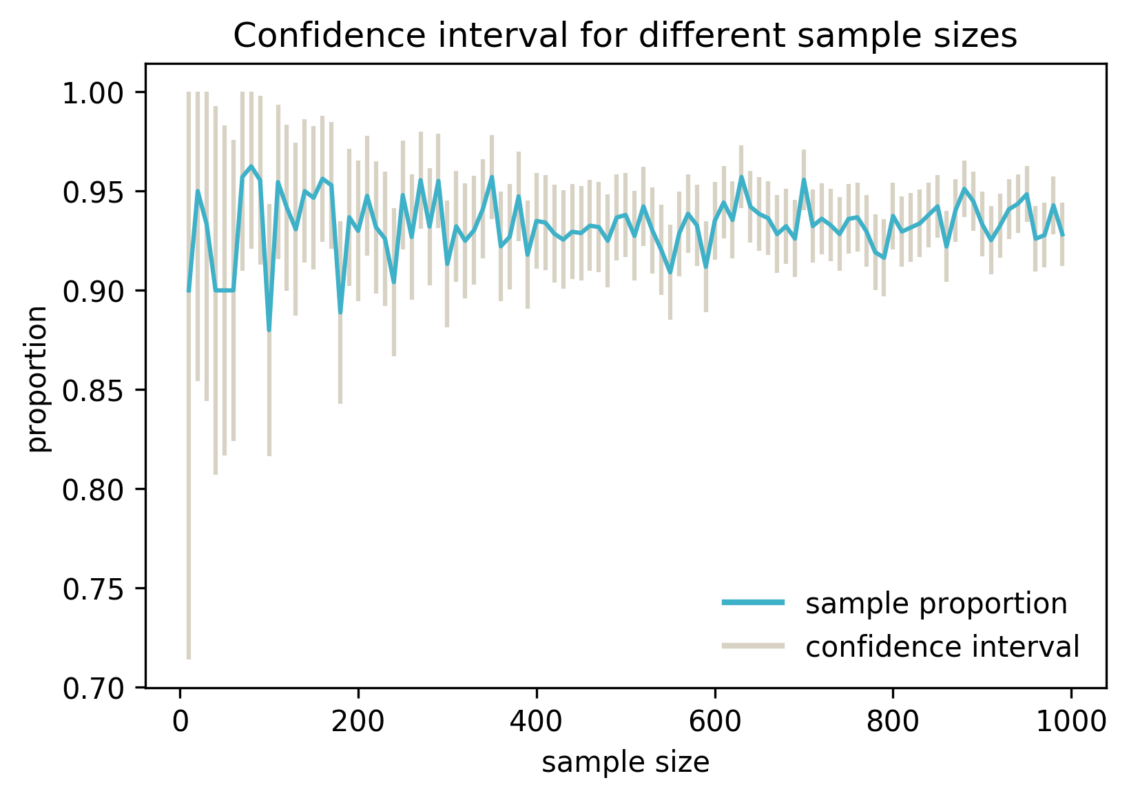
The blue line represents the estimated proportion for samples of different sizes, and the grey vertical lines are confidence intervals. The estimated proportion varies, because for each size a different sample was drawn.
We can see that increasing the sample size decreases the interval. This should make intuitive sense: if we have more data to estimate from, we can expect our estimate to be more reliable (i.e. closer to the population proportion).
What about the confidence level? By setting the confidence level we specify, how certain we want to be about our confidence interval. So far I used 95%. What happens if I calculate the confidence intervals for my original sample of 100 records, but with varying confidence level?
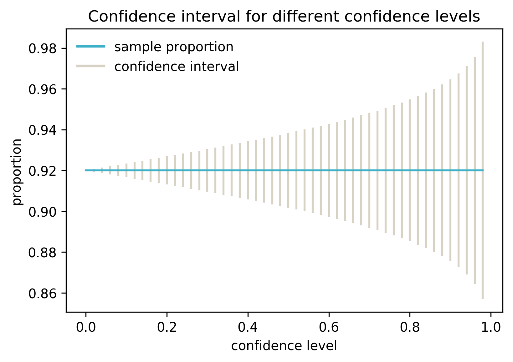
In this case the average is always the same, because only one sample was used.
As we can see, increasing the confidence level widens the interval. In other words, the more certain we want to be about the interval containing the real population average, the wider the interval has to be.
Sampling distribution
So far so good, but where does this magic confidence interval actually come from? It is calculated by the theoretical analysis of the sampling distribution (not to be confused with sample distribution):
- Sample distribution is when we collect one sample of size k and calculate a certain feature for every element in the sample. It is a distribution of k values of the feature in one sample.
- Sampling distribution is when we independently collect n samples, each of size k, and calculate the sample proportion for each sample. It is the distribution of n sample proportions.
Imagine I collect all samples of size 100 from my population and I calculate the sample proportion for each sample. This is the sampling distribution. Now I randomly choose one number from this sampling distribution. Note that this is equivalent to what I did before: choosing one random sample of size 100 and calculating its sample proportion.
According to Central Limit Theorem, sampling distribution is approximately normal with the mean equal to the population proportion. Here is the visualisation of the sampling distribution:
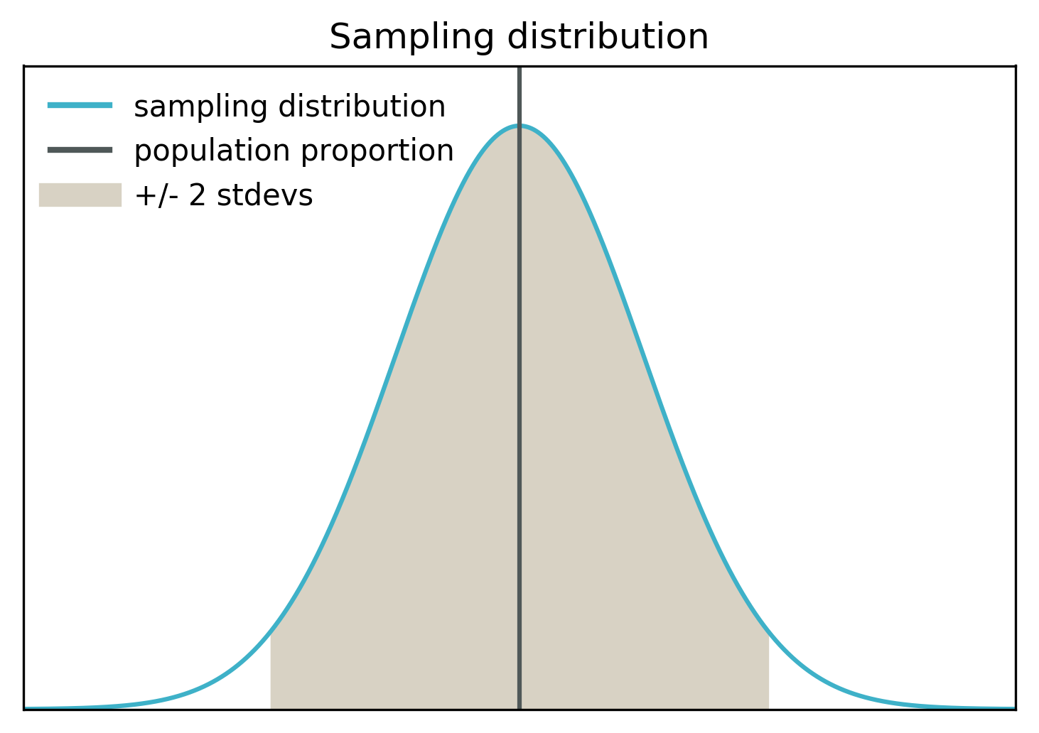
The black vertical line shows the mean of the sampling distribution. This is also the real population proportion. The grey area covers the middle 95% of the distribution mass (within 2 standard deviations from the mean).
When we choose one sample and calculate the sample proportion, there are two possibilities:
- With 95% probability, we were lucky and the sample proportion is within the grey area. In that case, the real population proportion is not further than 2 standard deviations from our estimate.
- With 5% probability, we were unlucky and the sample proportion is outside the grey area. In that case, the real population proportion is further than 2 standard deviations from our estimate.
So with the confidence of 95% we can say that the real population proportion is within 2 standard deviations from our sample proportion. We can see now that these 2 standard deviations of the sampling distribution define our confidence interval at the confidence level of 95%.
Smaller confidence level would make the grey area narrower, and the confidence interval would shrink as well. Larger confidence level makes the grey area, and the confidence interval, larger.
To look more closely at the sampling distribution, I generated sampling distributions for all combinations of “n samples of size k”, where n and k are the elements of the set {25, 50, 100, 200, 400, 800, 1600, 3200}. This is only an approximation, since the real sampling distributions would contain many more samples.
Here is the heatmap showing the mean of each sampling distribution (this should be approximately the same as the real population proportion):
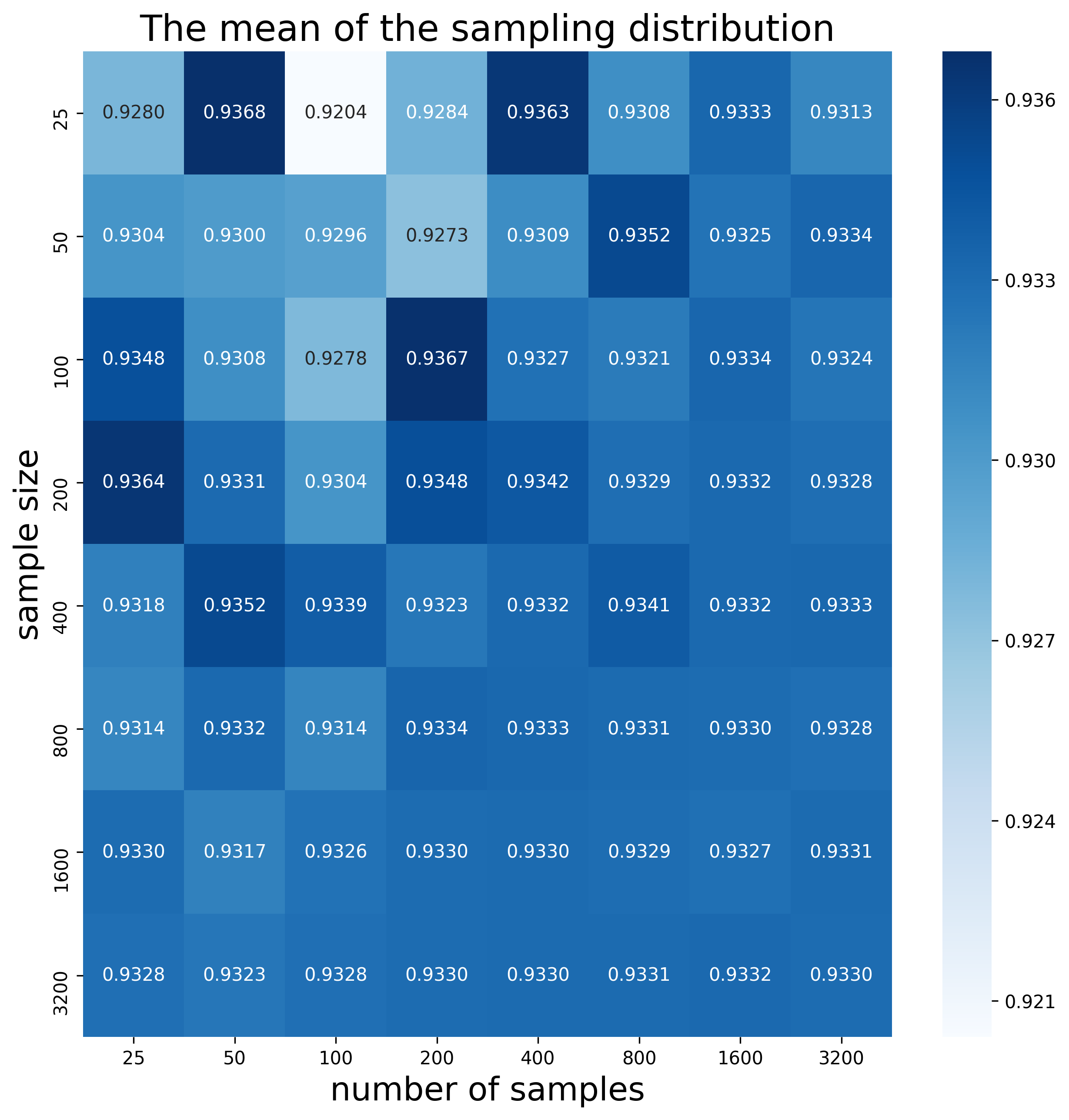
We can see that there is some variability in the top left part of the heatmap, which corresponds to small sample sizes and small numbers of samples. The bottom right part of the heatmap shows much less variability. As we increase the sample size and number of samples, the mean of the sampling distribution approaches numbers around 0.933.
Here is the heatmap showing the standard deviation for each sampling distribution:
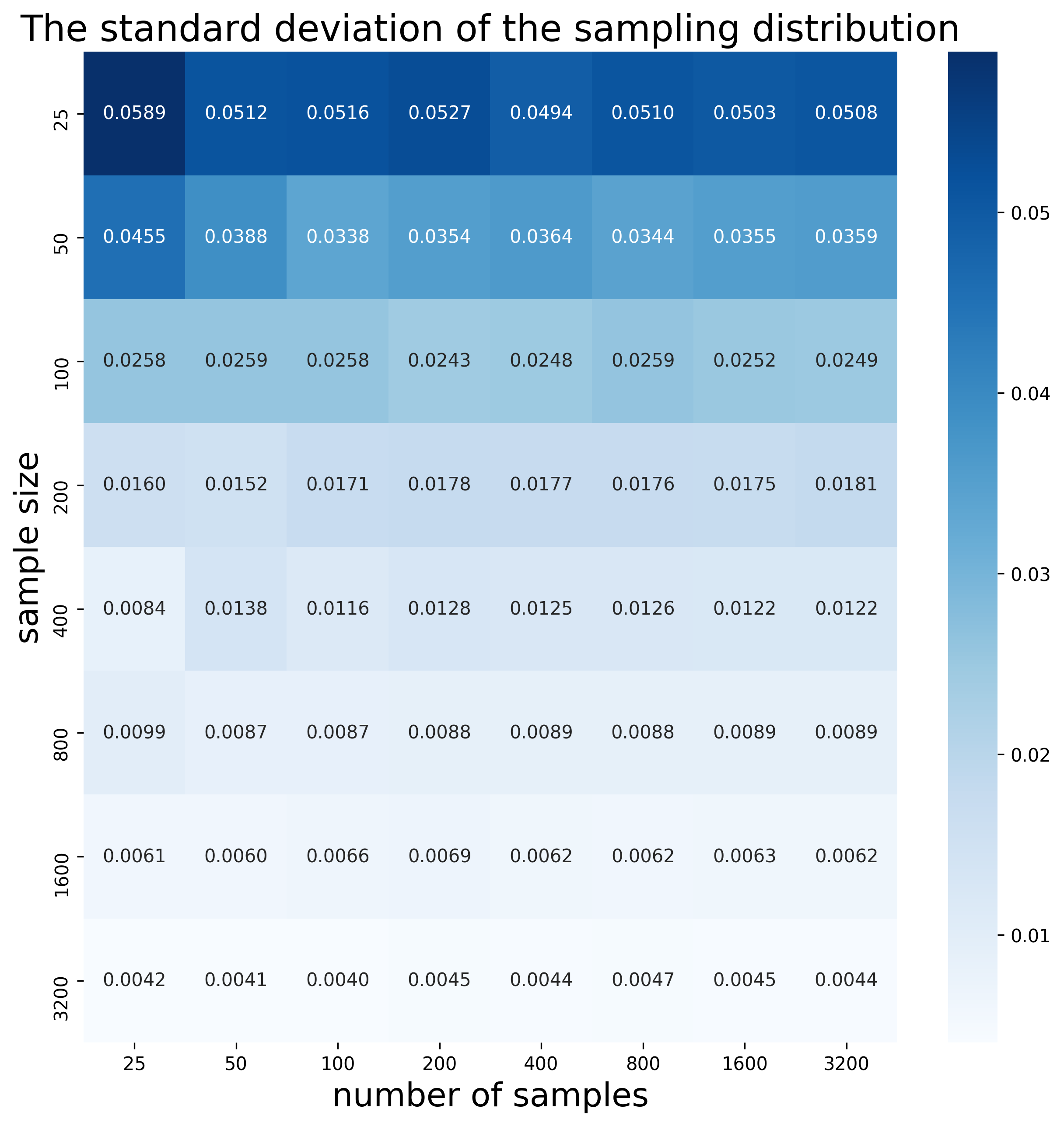
We can clearly see how the standard deviation decreases when we increase the sample size. This is consistent with the previous observation, that the confidence interval decreases when the sample size is increased.
Let’s also see the histograms of all the sampling distributions:
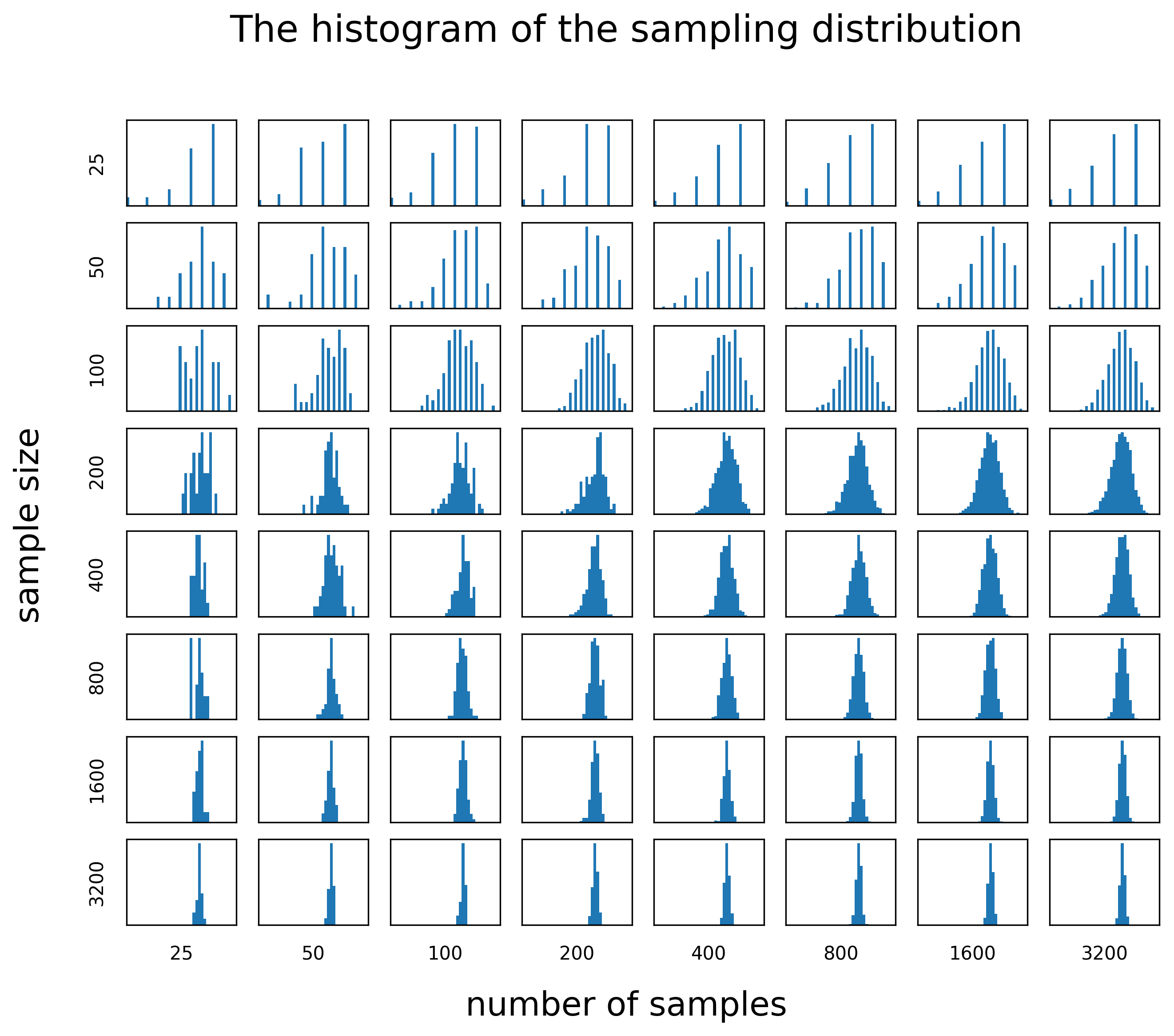
Here we can see the following patterns:
- All histograms indeed seem to be centered around approximately the same number.
- The more samples we include, the more normal the sampling distribution appears. This happens because with more samples the real sampling distribution is better approximated.
- The larger the sample size, the narrower the sampling distribution (i.e. smaller standard deviation).
The estimation vs. the real value
Let’s go back to my original question. What is the proportion of reference strings in APA style, that are successfully matched to the original DOIs of the records they were generated from? So far we observed the following:
- A small sample of 100 gave the estimate 0.92 (confidence interval 0.8668-0.9732)
- A larger samples of 1000 gave the estimate 0.932 (confidence interval 0.9164-0.9476)
- The means of sampling distributions seem to slowly approach 0.933
So what is the real population proportion in my case? It is 0.933005. As we can see, the estimations were fairly close, and the intervals indeed contain the real value.
Now I can also calculate the confidence interval for each sample in my sampling distributions, and then the fraction of the intervals that contain the real population proportion (I expect these numbers to be close to the confidence level 95%). Here is the heatmap:
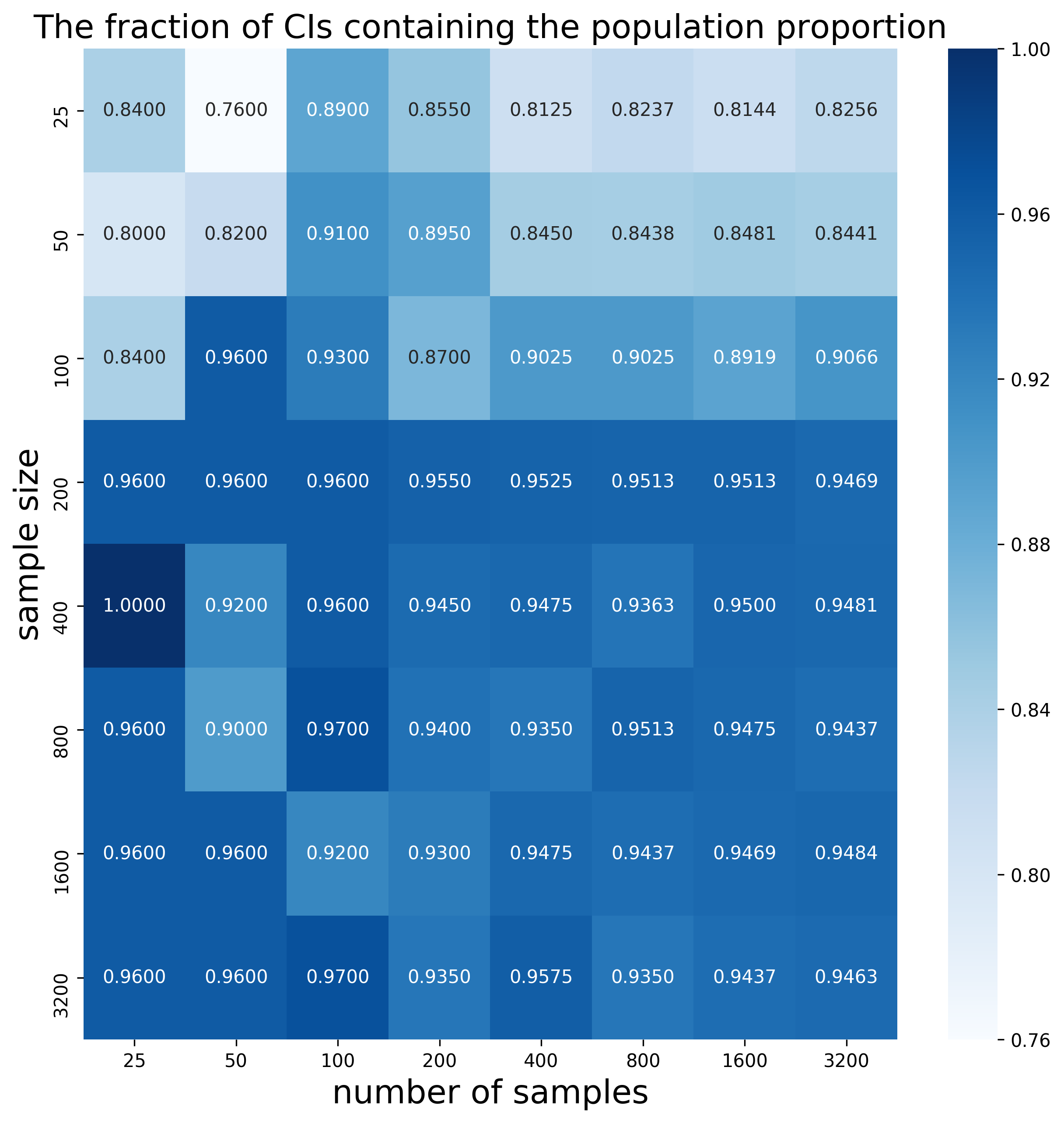
We can see that for larger sample sizes indeed the fractions are high. The fraction is not always above 95%, as we would expect, especially for smaller sample sizes. One of the reasons is that when we calculate the confidence interval, we approximate the standard deviation of the population with the standard deviation of the sample. This is not always a reliable estimate, especially for small samples. This suggests that sample sizes of at least 1000-2000 should be used.
Be careful
Some important things to remember:
- Aggregate functions. As mentioned before, apart from estimating the proportion, a similar procedure can be applied for estimating the average of a certain numeric feature.
- (Lack of) certainty. Remember that the confidence level < 1. This means that we are never sure that our confidence interval contains the true population proportion. If for any reason you need to be 100% sure, just process the entire dataset.
- Randomness, a.k.a. “stirring before tasting”. The sample has to be chosen randomly. Beware of assuming that the dataset is shuffled and taking the first 1000 rows!
- Sample size. We know already that the larger the sample, the better. As a rule of thumb, using sample sizes < 30 makes the estimates, including the interval, rather unreliable.
- Skewness. In general, the more skewed the original feature distribution, the larger sample we need. In case of the proportion, the sample should contain at least 5 data points of each value of the feature (passes/doesn’t pass the test).
- Generalization. The sample average/proportion can be used as an estimate for the population average/proportion, but only the population it was drawn from. This means that if we applied any filters before sampling (which is equivalent to sampling from a subset passing the filter), we can reason only about the filtered subset of the data.
- Reproducibility. This is more of an engineering concern. In short, all the analyses we do should be reproducible. In the context of sampling it means, at the very least, that we should record the samples we use.
Further reading
- Jul 8, 2019 – What if I told you that bibliographic references can be structured?
- Dec 18, 2018 – Reference matching: for real this time
- Nov 12, 2018 – Matchmaker, matchmaker, make me a match
- Mar 3, 2015 – Real-time Stream of DOIs being cited in Wikipedia
- Mar 2, 2015 – Crossref’s DOI Event Tracker Pilot
- Jan 12, 2015 – Introducing the Crossref Labs DOI Chronograph
- Mar 19, 2026 – On metadata enrichment
- Mar 22, 2022 – Follow the money, or how to link grants to research outputs