


Introduction
Polycrystalline ice deforms mainly by intracrystalline dislocation glide (Pimienta and others, 1987). The ice single crystal deforms essentially by slip on the basal plane, normal to the hexagonal symmetry c axis. Due to the strong anisotropy of the single crystal (Duval and others, 1983), strain incompatibilities arise in the ice polycrystal, resulting in a non-uniform stress field at the grain scale. In the upper part of a polar ice sheet, where the stress level is very low, fast grain-boundary migration associated with grain growth, which tends to lower the surface energy of the grains, is an efficient process to relieve the stress concentrations and might explain the low Newtonian viscosity derived from the analysis of inclinometry surveys (Lliboutry and Duval, 1985). With increasing depth and deviatoric stresses, grain growth vanishes as strain hardening becomes influential, and the main accommodation mechanisms are lattice rotation associated with polygonization of the grains which have a high stored energy, and grain-boundary migration (Alley, 1992; Alley and others, 1995; Duval and Castelnau, 1995). In this “rotation-recrystallization” regime, the rotation of the caxes of the grains induces the formation of a fabric (statistical distribution of the caxes), which evolves as a function of the strain history of the ice. Very strong fabrics, with alignment of the caxes along the vertical, or random distribution of the caxes in a vertical plane, have been observed in ice cores drilled at different sites in Antarctica and Greenland (Gow and Williamson, 1976; Russell-Head and Budd, 1979; Herron and Lang-way, 1982; Fujita and others. 1987; Lipenkov and others, 1989). Laboratory experiments (Bouchez and Duval, 1982; Wilson, 1982; Jacka and Maccagnan, 1984; Azuma and Higashi, 1985; Pimienta, 1987) and inclinometry analysis (Russell-Head and Budd, 1979; Shoji and Langway, 1984: Gundestrup and Hansen, 1984; Hansen and Gundestrup, 1988) have shown that these fabrics greatly influence the mechanical behaviour of ice and consequently the flow of the polar ice sheets. When approaching the bedrock, high temperature and relatively high fluctuating stresses initiate dynamic recrystallization, with fast grain-boundary migration, and the formation of a multi-maxima fabric which adapts to the local state of stress, as found in temperate glaciers. According to Duval and Castelnau (1995), this “migration-recrystallization” regime begins when the temperature reaches −12°C.
So far, only a few models have been published on ice anisotropy. The first model for describing the mechanical behaviour of ice for a given anisotropy was that of Lile (1978), who assumed a Newtonian behaviour for the ice single crystal. Lliboutry (1987) derived an anisotropic power law depending on seven parameters, under the assumptions that the stress is uniform and there is no energy dissipation at grain boundaries. Lliboutry (1993) extended his model to a polynomial flow law by adding a Newtonian dissipation potential (which increases the number of parameters to ten). As regards fabric development, a simple model for uniaxial compression was given by Azuma and Higashi (1985); it considers each crystal in the aggregate as an isolated crystal subject to a basal shear strain proportional to the overall strain and to geometrical constraints. Fujita and others (1987) and Pimienta (1987) extended this model to the case of uniaxial tension, then Alley (1988) to simple shear. A more elaborate and general version of this model has been developed by Azuma (1994). Models based on the hypothesis of a uniform stress slate in the polycrystal have been proposed by Van der Veen and Whillans (1994) and Castelnau and Duval (1994), the former including strain/stress induced recrystallization criteria. All these models are based on the assumption that a grain in a polycrystal reacts as if it were a single (isolated) crystal submitted to a basal shear stress which is postulated a priori.
More recently, in order to reject the assumption level closer to the physical mechanisms involved at the grain scale, Castelnau and others (in press) have used a powerful viscoplastic self-consistent (VPSC) model to simulate fabric formation and evolution in polar ice. This model considers each grain as a heterogeneous inclusion embedded in a homogeneous matrix which can exhibit any kind of anisotropy. It is assumed that the ice single crystal deforms by slip on the basal plane and on the prismatic and pyramidal planes. Contrary to the previous models, there is no need to make any assumption on the local state of stress or strain in a grain. The only basic hypothesis, independent of the assumed mechanical behaviour of the ice single crystal, is that the c-axis orientation of a grain does not depend upon the orientation of the neighbouring grains; this allows one to assume that all the grains with the same orientation are undergoing the same mean state of stress exerted by an equivalent homogeneous medium (HEM). The mechanical properties of the HEM derive from the mean response of all the grains to the applied conditions at the HEM boundary. This model reaches a high level of complexity and gives today, without any doubt, the most accurate results.
It can be questioned if, from a practical point of view, this model is well suited to dealing with ice-sheet modelling. To simulate the behaviour of a polycrystal (i.e. a material point in the flow domain), the model needs to consider a minimum of 100 grains; then solving a flow problem by finite elements (for instance) requires storage of at least 100 orientations at each integration point. If some degree of accuracy is needed (large number of elements and more than three integration points per element), the required storage capacity will be enormous, even for a two-dimensional problem. Moreover, the time needed for the computation of the texture development, at each integration point, will increase the difficulty of such a procedure. However, mean aggregate properties and fabric evolution deduced on this scale can suggest a suitable simplified continuum response for larger-scale applications.
Proposed Model
Main features and restrictions of the model
The model presented here is of the same nature as the VPSC model, but additional assumptions are made in order to achieve a simpler formulation which could be used for ice-flow modelling purposes.
The fabrics which are likely to have a significant influence on the flow of ice caps are strong fabrics with caxes clustered around the vertical, which form under compression and/or simple shear, and that with coplanar caxes, which form under extension. In the first case, the enhancement factor on the strain rates is about 10, whereas in the latter configuration, when the ice is loaded along the symmetry axis of the fabric, it is less than 0.1 (Pimienta and others, 1987). Taking into account these particular fabrics would be a major improvement of the existing ice-sheet models. Intermediate fabrics with two maxima, as observed by Bouchez and Duval (1982), can be modelled by Azuma (1994) and Castelnau and others (in press) but evolve towards a single-maximum fabric with increasing accumulated strain. Multi-maxima fabrics, found in the “migration-recrystallization” zone near the bedrock, cannot be modelled without including the recrystallization processes. However, laboratory experiments (Duval, 1981) and temperate-glacier flow simulations (Meyssonnier, 1989) have shown that an isotropic power law is quite convenient to model the mechanical behaviour of this ice.
To capture the essential features of the in-situ observed fabrics, we propose to model polar ice as a transversely isotropic medium. Rather than considering the ice polycrystal as an assembly of a discrete number of individual grains, we replace the discontinuous distribution of the orientations of the caxes with a continuous orientation distribution function (ODF), which gives the density of grains with a given orientation.
To allow analytical calculations, each grain of the polycrystal is modelled as a transversely isotropic medium, the symmetry axis of which is the caxis of the crystal, with a weak resistance to shear parallel to the basal plane. This reduction of the actual behaviour of the ice crystal may be justified as follows:
According to Kamb (1961), when a single crystal of ice deforms by simultaneous gliding along its three a axes, following a power law, the resultant gliding direction is exactly the same as that of the resolved shear stress on the basal plane if the exponent n of the power law is 1 or 3. For 1 < n < 3, the maximum deviation is of the order of 2°.
The mechanical behaviour of a grain in a polycrystal of ice differs significantly from that of a single (isolated) crystal undergoing the same state of stress; under stresses of the order of 1 MPa, basal glide in a single crystal follows a power law with n = 2, whereas at the same stress level the value of n for a polycrystal is 3. The strain incompatibilities between neighbouring grains activate mechanisms other than basal glide, probably dislocation climb rather than the activation of other glide systems (Duval and others, 1983), which control the mechanical response of the grains. Then, the phenomenological approach adopted here to model the behaviour of a grain is acceptable, since the classical approach used in polycrystal plasticity, involving a number of slip systems, does not seem to reproduce the actual mechanisms of ice deformation.
Further simplification is achieved, in this first version of the model, by assuming a Newtonian behaviour for the grains. This does not render the model inappropriate, as some indications of a power-law exponent less than 2 can be found in the literature (Doake and Wolff, 1985; Lliboutry and Duval, 1985; Pimienta, 1987). Extension to a more general (non-linear) behaviour is possible but this is left for future work.
The most severe limitation of the model, in its current form, is that it is restricted to loading conditions which respect the symmetry of the fabric.
General framework
The starling point is Eshelby’s relation for an elastic (homogeneous) ellipsoidal inclusion in an elastic matrix or HEM with a free boundary at infinity. If this inclusion ![]() were removed from the HEM, then unloaded, it would take the shape
were removed from the HEM, then unloaded, it would take the shape ![]() , leaving a hole of shape
, leaving a hole of shape ![]() 0 in the HEM. The transformation of
0 in the HEM. The transformation of ![]() 0 to
0 to ![]() * corresponds to a strain є* which is called the “stress-free strain” of
* corresponds to a strain є* which is called the “stress-free strain” of ![]() . According to Mura (1987), the displacement u inside the inclusion, corresponding to an imposed arbitrary stress-free strain є*, is
. According to Mura (1987), the displacement u inside the inclusion, corresponding to an imposed arbitrary stress-free strain є*, is
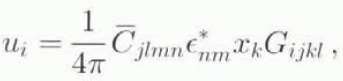
where ![]() is the stiffness tensor of the HEM, x are Cartesian coordinates in the reference frame defined by the (geometrical) principal axes of the inclusion, and the Gijkl
components are integrals, over the surface of the inclusion, which depend only on the elastic moduli of the HEM and on the inclusion-shape ratio.
is the stiffness tensor of the HEM, x are Cartesian coordinates in the reference frame defined by the (geometrical) principal axes of the inclusion, and the Gijkl
components are integrals, over the surface of the inclusion, which depend only on the elastic moduli of the HEM and on the inclusion-shape ratio.
Following Gilormini and Vernusse (1992), we use the results obtained by Mura (1987) for an ellipsoidal inclusion with a geometrical symmetry axis parallel to the symmetry axis of a transversely isotropic HEM. The major advantage of this approach is that the expressions for Gijkl can be integrated analytically. However, this is a further restriction on the model, and we will consider only the simplest case of spherical grains which are assumed to remain spherical during their deformation.
In the following, all macroscopic variables related to the HEM are overlined.
The displacement gradient inside the inclusion is derived from Equation (1) in the framework of infinitesimal strain and rotation. By applying the superposition principle, it follows that when the HEM is submitted to a prescribed strain ⋷ at infinity, corresponding to a stress ![]() , the strain ϵ in the inclusion is
, the strain ϵ in the inclusion is
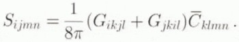
where S is the Eshelby’s tensor of components,
In order to satisfy static equilibrium, the stress σ in the inclusion must be
where I denotes the identity tensor.
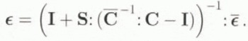
When considering a heterogeneous inclusion (inhomogeneity), the stress-free strain ϵ* is defined by Equations (2), (4) and the behaviour law of the inhomogeneity
After some algebra, the classical interaction formula is obtained as
The rotation tensor in the inhomogeneity, for a rotation ϖ prescribed at infinity on the HEM, is
where ω* is a consequence of the interaction between the inhomogeneity and the HEM. The components of ω* derive from Equation (1) as
where is the tensor of components
Using relations (7), (8) and (2), the rotation in the inclusion becomes
The aim of the following sections is to develop analytical forms for relations (6) and (10), then to apply these relations for ice by using the principle of correspondence.
Transverse isotropy
In the following, two Cartesian reference frames, ![]() and
and  , are used (see Fig. 1):
![]() is a fixed global frame whose
is a fixed global frame whose ![]() axis is the HEM symmetry axis.
axis is the HEM symmetry axis.
 is a local frame attached to a grain, whose z axis coincides with the caxis.
Any (non-scalar) quantity, expressed as x in ![]() , is noted as x
i
when expressed in
, is noted as x
i
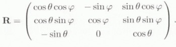
when expressed in  . The orientation of a grain is given by the two angles θ and ψ, defined in Figure 1.
The components a and a
<i
of the same vector with respect to ![]() and
and  are related by a = R · a
i
, with
are related by a = R · a
i
, with
Using Voigt’s notation (the stress and strain tensors are expressed as vectors; σ = {σ1, σ2, σ3, σ23, σ31, σ12}, ϵ = {ϵ1, ϵ2, ϵ3, 2ϵ23, 2ϵ31, 2ϵ12}), the elastic compliance of the transversely isotropic HEM. expressed in ![]() , is noted
, is noted
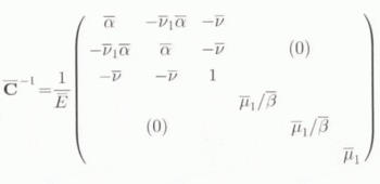
where ![]() . ᾱ is the ratio of the Young’s modulus Ē along the symmetry axis (
. ᾱ is the ratio of the Young’s modulus Ē along the symmetry axis (![]() in Figure 1) to that in the plane of isotropy (
in Figure 1) to that in the plane of isotropy (![]() , ӯ), ῡ and ῡ are the Poisson’s ratios in the planes parallel and perpendicular to the symmetry axis, respectively.
, ӯ), ῡ and ῡ are the Poisson’s ratios in the planes parallel and perpendicular to the symmetry axis, respectively. ![]() is the ratio of the shear modulus in a plane which contains the symmetry axis to that in the plane of isotropy
is the ratio of the shear modulus in a plane which contains the symmetry axis to that in the plane of isotropy ![]() .
.
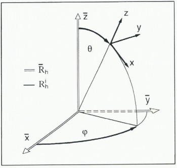
Fig. 1. Macroscopic ![]() , and grain
, and grain ![]() , Cartesian reference frames; angles λ and ψ define the c-axis orientation of a grain.
, Cartesian reference frames; angles λ and ψ define the c-axis orientation of a grain.
The elastic compliance of the inhomogeneity expressed in ![]() , takes a similar form in which Ḕ, ᾱ,
, takes a similar form in which Ḕ, ᾱ, ![]() ,
, ![]() , ῡ1, ῡ, are replaced with E, α, β, μ. ν1, ν.
, ῡ1, ῡ, are replaced with E, α, β, μ. ν1, ν.
Incompressibility
Incompressibility is obtained by prescribing the values of ν, ῡ, ν1 and ῡ as
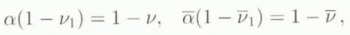
so that
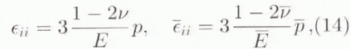
where p and ![]() denote the isotropic pressures in the inclusion and the HEM, then letting ῡ = ν approach 1/2. The analytical expressions for the Eshelby’s tensor components, at order zero in the small parameter 1 – 2ν, can be found in Gilormini and Vernusse (1992), who studied the case of an isotropic incompressible inhomogeneity in a transversely isotropic HEM. Taking the general symmetry relations into account, the non-zero components of S are
denote the isotropic pressures in the inclusion and the HEM, then letting ῡ = ν approach 1/2. The analytical expressions for the Eshelby’s tensor components, at order zero in the small parameter 1 – 2ν, can be found in Gilormini and Vernusse (1992), who studied the case of an isotropic incompressible inhomogeneity in a transversely isotropic HEM. Taking the general symmetry relations into account, the non-zero components of S are
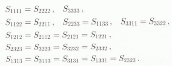
Additional relations which are useful to achieve results in closed form are
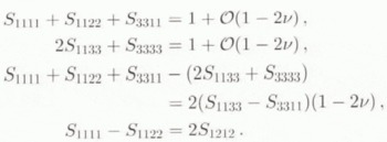
The expressions for the Sijkl are given in the Appendix.
Interaction formulae for the ice polycrystal
The results obtained for elastic behaviours of the inhomogeneity and the HEM can be transposed to linearly viscous materials, of axial viscosities η and ![]() along the respective symmetry axes, by imposing incompressibility and replacing the strain ϵ with the strain rate ⋵, the rotation ω, with the rate of rotation
along the respective symmetry axes, by imposing incompressibility and replacing the strain ϵ with the strain rate ⋵, the rotation ω, with the rate of rotation ![]() , the stress σ with the deviatoric stress s, and the Young’s moduli E and Ē with 3η and 3
, the stress σ with the deviatoric stress s, and the Young’s moduli E and Ē with 3η and 3![]() , in relation (5)–(12). This is valid for infinitesimal strains and rotations from the current state and hence determines the instantaneous response from any deformed state.
, in relation (5)–(12). This is valid for infinitesimal strains and rotations from the current state and hence determines the instantaneous response from any deformed state.
Matrix ![]() given by relations (12) is now a viscosity matrix, and macroscopic parameter ᾱ is the ratio of the axial viscosity
given by relations (12) is now a viscosity matrix, and macroscopic parameter ᾱ is the ratio of the axial viscosity ![]() along the symmetry axis (
along the symmetry axis (![]() axis) of the ice polycrystal (HEM) to the axial viscosity
axis) of the ice polycrystal (HEM) to the axial viscosity ![]() in the plane of isotropy (i.e., the viscosity which would be measured in uniaxial compression along the
in the plane of isotropy (i.e., the viscosity which would be measured in uniaxial compression along the ![]() or ӯ axis). Macroscopic parameter
or ӯ axis). Macroscopic parameter ![]() is the ratio of the shear viscosity
is the ratio of the shear viscosity ![]() in the
in the ![]() or (ӯ−
or (ӯ−![]() ) plane to the shear viscosity
) plane to the shear viscosity ![]() in the plane of isotropy. This is summarized by
in the plane of isotropy. This is summarized by
The same definitions apply to the grain (inclusion) parameters η, α and β.
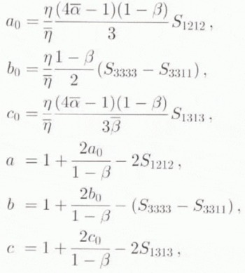
The development of relation (6), using relations (12), expressed in frame ![]() , and relations (13)–(16), is lengthy but straightforward. Additional simplification was obtained by making α = 1 in the grain-behaviour form of relation 112); this does not conform to Pimienta’s (1987) results but preserves the essential feature of the grain behaviour (i.e., a weak resistance to shear parallel to the basal plane, obtained with β < 1). The corresponding form of relation (17) for the grain is then
, and relations (13)–(16), is lengthy but straightforward. Additional simplification was obtained by making α = 1 in the grain-behaviour form of relation 112); this does not conform to Pimienta’s (1987) results but preserves the essential feature of the grain behaviour (i.e., a weak resistance to shear parallel to the basal plane, obtained with β < 1). The corresponding form of relation (17) for the grain is then
By using the correspondence principle and separating the isotropic and deviatoric parts, the resulting interaction formulae, expressed in ![]() , give the strain rate ⋵ and the isotropic pressure p in a grain of c-axis orientation (θ, φ), as a function of the strain rate
, give the strain rate ⋵ and the isotropic pressure p in a grain of c-axis orientation (θ, φ), as a function of the strain rate ![]() and of the isotropic pressure
and of the isotropic pressure ![]() in the HEM. They are
in the HEM. They are
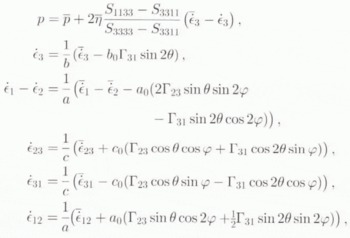
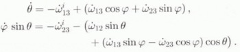
where
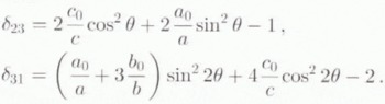
and Γ23. Γ31 are the expressions for the shear-strain rates ![]() and
and ![]() in the grain, expressed in
in the grain, expressed in  by
by
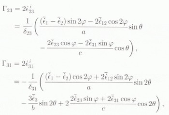
with
Self-consistency
To describe the fabric, we use an QDF (Orientation Distribution Function) f(θ, φ), which gives the density of caxes with orientation (θ, φ), i.e. the relative number of caxes intersections with the unit sphere per unit area of the sphere. The relative number of grains whose orientations lie in the interval (θ, θ + dθ; φ, φ + dφ) is
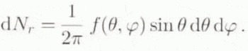
Assuming that there is no correlation between the volume of a grain and its orientation, dN r is also a volume fraction.
By definition,
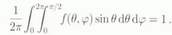
For a transversely isotropic HEM, f does not depend on φ, i.e., f(θ, φ) = f(θ). The weighted average of a quantity x(θ, φ) is then defined as
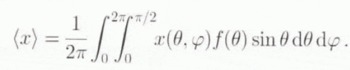
For an isotropic HEM: f(θ, φ) = 1.
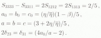
The self-consistency of the model is achieved by setting the averages of the isotropic pressure and of the strain rates equal to their corresponding macroscopic quantities, that is
Using expressions (19) for p and ⋵
ij
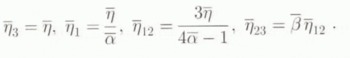
, with the complementary relations (15), (16) and (20)–(22), relations (25) and (26) result in the following non-linear set of three equations for the unknowns ![]() , ᾱ,
, ᾱ, ![]() :
:
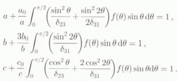
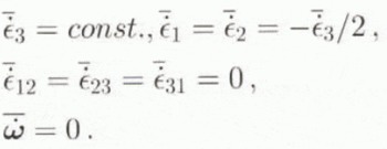
The solution of Equation (27) can only be found numerically, except for the simple isotropic fabric. In this case ᾱ = ![]() = 1 and the following relations hold:
= 1 and the following relations hold:
Then system (27) reduces to the equation (3)( –2β = 0, which has only one positive root
 ![]() given by
given by

Thus, for small values of β, the macroscopic viscosity of the HEM is controlled In the main viscosity along the c-axis direction.
Fabric evolution
According to Equation (11), the components c and c i of the c-axis vector of a grain are linked by
Under the velocity gradient L in the grain, c transforms into c + dc such that
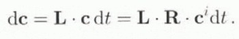
Differentiating Equation (30) with respect to time leads to
It follows that
By introducing the rate of rotation tensor ![]() , defined by L = ⋵ +
, defined by L = ⋵ + ![]() , and using the transformation formula ⋵ = R η
, and using the transformation formula ⋵ = R η ![]() i
η R
−1, expression (11) for R and c
i
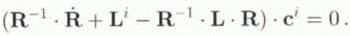
= ͻ0, 0, 1ͽ, the change in the orientation of a grain follows from Equation (33) as
i
η R
−1, expression (11) for R and c
i
= ͻ0, 0, 1ͽ, the change in the orientation of a grain follows from Equation (33) as
Assuming that the basal planes of a grain remain parallel to each other during the deformation, the component of the velocity in a grain along the z axis (caxis) is a function of z only, so that
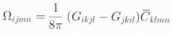
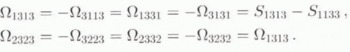
The components of the rate-of-rotation tensor in the global reference frame ![]() are given by Equation (10) (written for rates). The Ω
ijkl
components which appear in this equation, not given by Gilormini and Vernusse (1992), need to be calculated from relation (9) and Mura’s (1987) expressions for the Gijkl
. For a transversely isotropic HEM, the only non-zero components are
are given by Equation (10) (written for rates). The Ω
ijkl
components which appear in this equation, not given by Gilormini and Vernusse (1992), need to be calculated from relation (9) and Mura’s (1987) expressions for the Gijkl
. For a transversely isotropic HEM, the only non-zero components are
From Equation (10) and (36), the non-zero components of ![]() in
in ![]() are
are
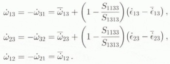
Using Equation (35), (37) and the interaction formulae (19)–(22) in relations (34), completely determines ![]() and
and ![]() .
.
The ODF evolution derives from the continuity Equation (24), by requiring that the net flux of grains which enters the interval (θ,θ + dθ; φ, φ + dφ) during a unit time is equal to the increase in the number of grains in this time, i.e.
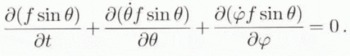
This equation, associated with Equation (34), describes the evolution of the fabric.
Application to Compression and Tension
Calculation procedure
The equations to be solved are the self-consistent system (27), which gives the mechanical behaviour of the HEM ![]() , and Equation (38) for the evolution of the ODF, using Equation (34).
, and Equation (38) for the evolution of the ODF, using Equation (34).
Under uniaxial compression or tension along the HEM symmetry axis, the velocity gradient prescribed at infinity, on the HEM boundary, is such that
Under these conditions, Equation (34) simplifies to

As Γ31 does not depend on φ, these equations confirm that the symmetry is maintained when compression, or tension, is exerted along the symmetry axis of the HEM.
Even though the present model is only valid for small strain and rotation, in this uniaxial geometry with no macroscopic rotation, a finite uniaxial strain can be reached by summing the small strain increments which arise in small time increments. The results can only be achieved by numerical computation, as the self-consistent set of Equation (27) is non-linear and the ODF is not explicated analytically. Starting from an isotropic configuration (f(θ) = 1, = 1), system (27) was solved by Newton’s method which was found to be always convergent. At the end of each time step, the macroscopic parameters ![]() , ᾱ
, ᾱ ![]() s, then the components of Eshelby’s tensor and the ODF were updated. Solution of Equation (38) was achieved by discretizing f(θ), then balancing the net flux of grains entering each interval (θ, θ + dθ) during the time step dt with the increase in f(θ) by using an upwind scheme which takes into account the sign of
s, then the components of Eshelby’s tensor and the ODF were updated. Solution of Equation (38) was achieved by discretizing f(θ), then balancing the net flux of grains entering each interval (θ, θ + dθ) during the time step dt with the increase in f(θ) by using an upwind scheme which takes into account the sign of ![]() at the ends of each θ interval.
at the ends of each θ interval.
Results
figure 2a, and b shows the evolution of the ODF, under compression and tension, respectively, as a function of the equivalent strain  . This equivalent strain has no physical meaning, as the model does not hold for finite strain, but it is a convenient reference measure for intercomparison between different models. As expected, the caxes tend to gather around the compression axis, or to fall in the plane perpendicular to the direction of tension, respectively, with increasing equivalent strain. As the relative number of grains in the interval (θ,θ + dθ) is f(θ) sin θ dθ (see Equation (23)), the usual representation of these fabrics by a Schmidt’s diagram would be two girdles, the radii of which decrease or increase respectively, with increasing equivalent strain. These curves were computed with β = 0.04 which is the solution of
 ![]() , with
, with ![]() given by Equation (29). With such a value of β, according to Equation (18), a polycrystal with all its caxes parallel, undergoing simple shear parallel to the basal plane of the grains, would deform ten times faster than an isotropic polycrystal, in accordance with Pimienta and others’ (1987) estimate (all other directional viscosities being equal to that of a grain along its symmetry axis).
given by Equation (29). With such a value of β, according to Equation (18), a polycrystal with all its caxes parallel, undergoing simple shear parallel to the basal plane of the grains, would deform ten times faster than an isotropic polycrystal, in accordance with Pimienta and others’ (1987) estimate (all other directional viscosities being equal to that of a grain along its symmetry axis).
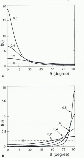
Fig. 2. Orientation distribution function f(θ) computed for different values of ![]() , with grain parameter β = 0.04. under (a) uniaxial compression, (b) uniaxial tension.
, with grain parameter β = 0.04. under (a) uniaxial compression, (b) uniaxial tension.

Fig. 3. Evolution of the macroscopic parameters ![]() , as a function of the equivalent strain ϵeq, for grain parameter β = 0.04, under (a) uniaxial compression, (b) uniaxial tension.
, as a function of the equivalent strain ϵeq, for grain parameter β = 0.04, under (a) uniaxial compression, (b) uniaxial tension.
The evolution of the mechanical parameters ![]() , and
, and ![]() , are shown on figure 3a and b. Under compression, in the extreme case of aligned caxes, the behaviour of the polycrystal should be that of the isolated grain (i.e.,
, are shown on figure 3a and b. Under compression, in the extreme case of aligned caxes, the behaviour of the polycrystal should be that of the isolated grain (i.e., ![]() ). This final state seems difficult to reach:; it ϵeq = 1, the macroscopic parameters are found to be
). This final state seems difficult to reach:; it ϵeq = 1, the macroscopic parameters are found to be ![]() . Taking the viscosity of the isotropic polycrystal as a reference, the corresponding viscosities at ϵeq = 1 are, according to Equation (17):
. Taking the viscosity of the isotropic polycrystal as a reference, the corresponding viscosities at ϵeq = 1 are, according to Equation (17):  . Under tension, in the extreme case of coplanar caxes, the viscosity along the polycrystal symmetry axis tends towards the axial viscosity of the grain. At ϵdq = 1, the macroscopic parameters are
 ![]() , and the corresponding viscosities are:
, and the corresponding viscosities are:  .
.
The influence of the grain parameter β on the evolution rate of the fabric, under uniaxial compression, is shown in figure 4a. The influence of β on the mechanical parameters of the HEM is shown in figure 4b; the stronger effect is on ![]() . Note, however, that at an equivalent strain of 1, the values of
. Note, however, that at an equivalent strain of 1, the values of ![]() computed for β = 0.1 and β = 0.01 are only in a ratio of 3, so that this influence is not too great.
computed for β = 0.1 and β = 0.01 are only in a ratio of 3, so that this influence is not too great.
ODF Parameterization
All of these results were obtained by discretizing the ODF on 90 intervals between 0 and π/2. By doing so, there is little advantage in using an ODF formulation rather than discretizing the polycrystal in a finite number of grains, as has been done in Castelnau and others (in press) model. To remedy this situation, an attempt was made to parameterize the ODF with a small number of parameters. By analogy with the results of Giessen and Houtte (1992), who derived analytical formulations for the ODF in a model based on Taylor’s assumption, it was found that, both in compression and tension, the present ODF can be very accurately fitted with a function of the form
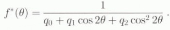
A theoretical demonstration of this, in the framework of the present model, is not straightforward, as the coefficients in Equation (40) for ![]() depend on ᾱ and
depend on ᾱ and ![]() which are implicit functions of f(θ).
which are implicit functions of f(θ).
The ODF’s obtained, with an evolving discretization of the ODF, or by using approximation (41) at the end of each time step to replace the actual ODF with f*, then discretizing f* at the beginning of the next time step (which mimics what should be done during a flow simulation), are practically identical, either under compression or tension, even at a large equivalent strain.
The generalization of such a parameterization, for loading conditions other than compression or tension, will retain the storage capacity required to solve a flow problem to a minimum.
Conclusion
An attempt to construct a simple model for the evolution of the anisotropy in polar ice has been made. The phenomenological approach has been limited to the description of a grain, in a polycrystal, as a transversely isotropic medium exhibiting linear viscous behaviour and weak resistance to shear parallel to the basal plane (general VPSC models restrict the phenomenological description to that of a gliding relation on crystallographic planes). Current ongoing work is attempting to achieve interaction formulae in closed form for a more elaborate model of a grain (non-linear behaviour and α ≠ 1). The additional assumptions or restrictions which were made, mainly considering a transversely isotropic polycrystal allowed analytical relations which give the state of strain acting at the grain level, while preserving the theoretical framework of the self-consistent method which has served as a good guideline.
In its current form, the model provides the mechanical parameters which describe the viscous behaviour, at time t and for a given (fixed) fabric, of a transversely isotropic polycrystal submitted to any velocity gradient at infinity. It can also predict the evolution df(θ, φ) of the ODF which represents the fabric but only for a (short) time step dt. In that sense, the model gives the tangent behaviour of this polycrystal.
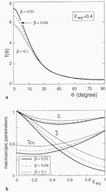
Fig. 4. Sensibility of the model to grain parameter β, under uniaxial compression: (a) computed ODFs f(θ) at ϵeq = 0.4; (b) macroscopic parameters ![]() .
.
Applications of the model, for boundary conditions which preserve the transverse isotropy of a polycrystal (compression, tension), have been presented.
Further work is needed to see how the ODF, f1 + df, which results from a strain increment applied to a transversely isotropic polycrystal with boundary conditions which do not preserve the symmetry, could be “symmetrized” at t + dt, that is, how an approximate transversely isotropic HEM (whose symmetry axis would differ from that at time t) could be found.
Acknowledgements
We greatly acknowledge Professor L. W. Morland, Drs B. Svendsen and R. Greve for their very helpful comments and discussion. Special thanks are due to Professor L. W. Morland, who generously gave his time to improve the quality of our English.
Appendix
Eshelby’s Tensor for an Incompressible Transversely Isotropic Medium
The Sijkl components derive form relation (3) in which the Gijkl for an ellipsoidal inclusion in a transversely isotropic medium have been given bu Mura (1987, p. 139–40), The results for an incompressible medium and any inclusion-shape ratio, at order zero in the small parameter (1–2ν) have been given by Gilormini and Vernusse (1992).
The expressions for a spherical inclusion are:
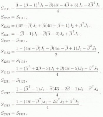
where
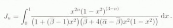
The other non-zero components derive from


