Introduction

After coring at Dome C, Antarctica, to a depth of 905 m in 1977–78 (Reference Lorius and DonnouLorius and Donnou 1978), temperatures were measured in the bore hole at 15 points. A more detailed temperature profile was obtained in 1978–79. Both will be analysed in this paper. Since probably, during the years to come, many temperature profiles in polar ice sheets will be obtained, still without accurate surface velocities or ages, it was worth examining all the information which may be retrieved from such temperature profiles.

Throughout this article the x-axis will be put at the ice-bedrock interface, in the direction of flow, and the z-axis upwards. Let u and w be the corresponding velocities and H the ice-sheet thickness, after replacing the firn by an ice layer of the same weight. Subscripts s denote surface values, subscripts b bottom ones.

The classical way of handling this problem is to set down a simple analytical expression for w(x,z), involving one or two unknown parameters, and to compute the corresponding temperature profile T(z). For instance:

(Reference RobinRobin 1955),

(Reference Budd, Jenssen and RadokBudd and others 1970),

(Reference Budd, Jenssen and YoungBudd and others 1973).

In the very cold upper layers, u = u(x) only, whence , and

(1)

(Reference Dansgaard and JohnsenDansgaard and Johnsen 1969, Reference Homer and GlenHammer and others 1978).

The parameter h in expression (1) has been estimated by Reference LliboutryLliboutry (1979), assuming u≫w and a bottom below freezing point. For a cold ice sheet of gently varying thickness, Lliboutry's formula (equation 51 in the above-mentioned paper) is:

(2)

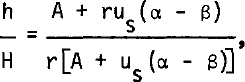
A being the accumulation (in equivalent height of ice), u_s the surface forward velocity, α and β the slopes of surface and bedrock, respectively, and (n is the exponent in Glen's creep law (n = 3), Q the activation energy for ice creep, R the gas constant, and G the geothermal gradient in stagnant ice (G ≃ 0.02 deg m⁻¹)).

When α = β = 0, this formula reduces to h ≈ H/r. For Dome C, r ≈ 10.8. Unfortunately, in our case, the bore hole is at an ice divide, where w and u are of the same order of magnitude, and normally this relation does not hold. Thus, a complete calculation of the coupled fields of velocities and temperatures must be done.

Near an ice divide, the horizontal advection of heat, its horizontal diffusion, and the viscous heat generation are negligible. With Cp denoting the heat capacity per unit volume, K the thermal conductivity, primes denoting derivatives with respect to z, and overdots time derivatives, the heat equation is:

(3)

The first objective, then, is to deduce T'(z) from the field measurements. We shall see that only a constant, mean value of T" in the bore hole can be confidently reached.

Next, a simplified calculation of both temperature and velocity fields, in the steady case, will be performed. It will give us an estimate of h, and of the bottom temperature.

Third, using relations (1) and (3), the temperature response of the ice sheet to a step function in T_s will be calculated. A time derivative will give us the response to a Dirac impulse for T_s, i.e. the impulse response R(z, t). Since past surface temperatures T_s(t) are known from ¹⁸0 measurements, the transient profile of temperatures can then be calculated by convolving T_s(t) and R(z, t), whence Ṫ.

Lastly, the actual vertical velocity can be deduced from relation (3). Since the mean accumulation A during recent centuries is known, the change in thickness of the ice sheet will ensue:

(4)

Field temperature profile and its derivatives

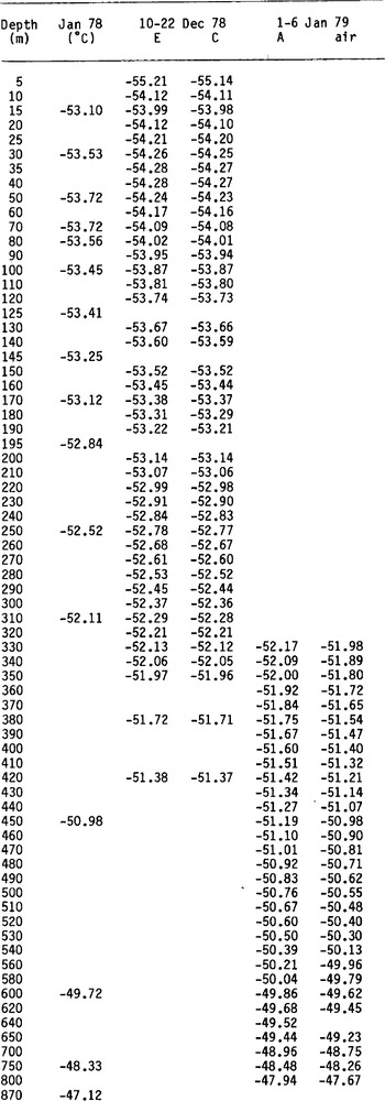
Temperature sensors were VECO 31A52 thermistors, embedded within copper bodies, in order to make self-warming during measurements negligible. A device pressed the copper bodies against the walls of the bore hole, and two disks of silicone rubber isolated the portion of hole where the measurement was made. Below 330 m, the air temperature 1n this closed chamber was also measured. The difference fluctuates between 0.20 and 0.27 deg. Since the objective is to measure temperature differences of about 0.08 deg for two points 10 m apart, the habitual method of merely measuring air temperatures in the bore hole must be excluded.

All field data are given in Table I. Below 650 m, only a few points, each 50 m, could be obtained, because of the fast closure of the empty bore hole. The very constant difference between the temperatures given by each sensor shows that temperature intervals are accurate to 0.01 deg. The inaccuracy comes principally from the field voltmeter which was used (Schlum-berger 7040). Calibration was done in Grenoble with a more precise one (DANA 5330, accuracy 10⁻⁵ instead of 20 × 10⁻⁵) and a standard of temperature Tinsley 5187 SA. Although this standard has a theoretical accuracy of 0.001 deg, constant differences of 0.01 deg between sensors C and E, and of 0.04 deg between sensors C and A were observed in the field.

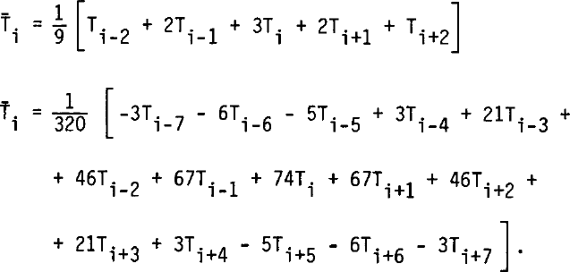
Values of T'(z) are given on Figures 1 and 2. In order to suppress noise, temperature values 10 m apart were smoothed by weighted running means (of 5 or 15 terms) which are almost perfect low-pass filters:

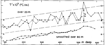
Fig.1 Temperature gradient over 20 m, as measured at Dome C bore hole. Below: running weighted means of five values. Solid line: at odd decametres; dashed line: at even decametres.

Oscillations of T' by a few per cent, with a wavelength of about 100 m, were found, identical in both cases. On Figure 2, the temperatures every 20 m, for even and odd decametres, have been handled separately. Weighted means over five successive terms then give oscillations which are in phase below 400 m and opposite above. Thus these oscillations, and the oscillating value for T" which may be deduced, have no physical meaning. (We hope this misadventure will make geophysicists who work only with smoothed data cautious!)

The general trend for T' is linear. A least-square fit gives T" = (3.63 ± 0.2) x 10⁻⁶ deg m⁻² between 100 and 520 or 630 in (Fig.1), and T" = 4.0 × 10⁻⁶ deg m⁻² between 75 and 825 m (Fig.2).

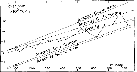
Fig.2 Temperature gradients over 50 m, compared with theoretical values for the steady state. A: accumulation; G: geothermal gradient in motionless ice.

Table I Measured Temperatures in the Dome C Bore Hole

Calculation of theoretical velocities and temperatures at an ice divide in the steady case

We assume the problem to be two-dimensional, with x = 0 as symmetry axis. This assumption is realistic, since Dome C is an elongated shoulder rather than a true dome. The bedrock is assumed to be a horizontal plane (z = 0), since its slope remains within the range (- 0.1 to + 0.1), and we are only interested in the upper layers of the ice sheet.

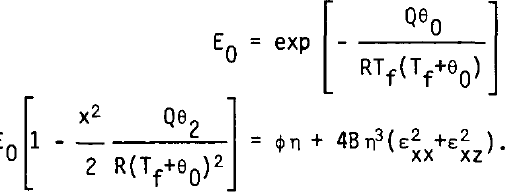
The main unknown is ice rheology, since it depends strongly on ice fabrics. In this calculation we adopt Glen's law for tertiary creep of ice, when the peculiar ice fabric, with four maxima of c-axis (as found in active ice near the melting point), has been formed (Reference DuvalDuval 1981). Nevertheless, to avoid numerical instability, a Newtonian viscous term (which may indeed exist) has been added. The temperature dependence is introduced by an Arrhenius factor, the same for both terms, although the apparent activation energy Q is known to increase above -10°C. The viscosity n is then given by:

(5)

where T_f. is the temperature at the melting point

(6)

μ being 1/1503 deg m⁻¹.

According to Reference DuvalDuval (1981), B = 0.1 bar⁻³ a⁻¹. A value Q = 60 kJ mol⁻¹ has been adopted, which is nearer to Reference PatersonPaterson's (1977) field value (54 kJ mol⁻¹) than to Reference Homer and GlenHomer and Glen's (1978) experimental one (75 kJ mol⁻¹). As for the Newtonian fluidity ϕ, it should be less than 0.01 bar⁻¹ a⁻¹ in order to become negligible in Duval's laboratory experiments.

Boundary conditions are: at the surface, no stresses against the surface, a uniform velocity w_s = -A, and a constant temperature T_s, and, at the bottom, either cold conditions (T_b < T_f), the thermal gradient T' having a given value G, with no sliding (u_b = W_b = 0), or temperate conditions (T_b = T_f), with W_b given by the energy balance, and U_b by the following sliding law:

(7)

This law would be found on a smooth sine profile, without ice-bedrock separation. The first term accounts for the melting-regeiation process, and for the Newtonian viscosity; the second one accounts for the plastic deformation.

Lateral boundary conditions are the most difficult to introduce. There do not exist regions on both sides where stresses could be considered as independent of x. A large number of mesh points along a horizontal would lead to huge calculations on a big computer, which our very crude rheological law and two-dimensional assumption do not deserve. Moreover, we are interested in the values for x = 0 only.

Thus, only three horizontal mesh points are taken, which means that all functions are approximated by odd or even polynomials in x with two terms only. Notwithstanding, in order to obtain the finite difference equivalent (in x) of the generalized biharmonic equation, the mean stress σ̅ = (σ_x + σ_Z)/2 must be approximated by a polynomial with three terms. Let us write, then (q denoting the stream function):

(8)

where the f_i, θ_i, n_i σ̅_i are functions of z.

The deviatoric stresses are then:

(9)

Equating in the equilibrium conditions (where ρg denotes the specific weight of ice):

(10)

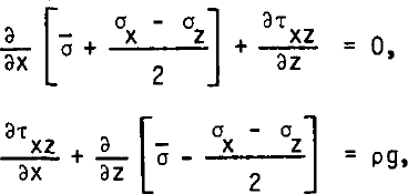
coefficients in like powers of x, the following five differential equations in z only are obtained:

(11)

(This first relation, which would enable a computation of σ₀, hence of σ_x and σ_Z, is useless for our purposes.)

(12)

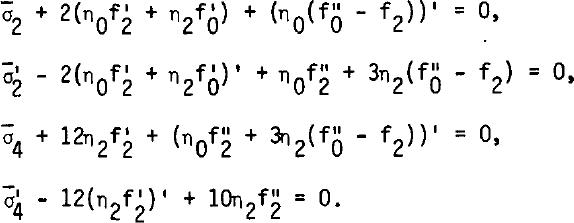
By eliminating σ̅₂ and σ̅₄, two coupled ordinary differential equations of the fourth order in f₀ and f₂ are found.

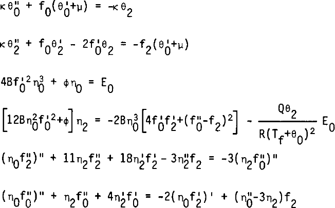
In a similar way, the heat equation in the steady case:

(13)

where K = K/C_ρ is the thermal diffusivity, affords two coupled ordinary differential equations of the second order in θ₀ and θ₂. Lastly, the viscosity is deduced from Equation (5), which becomes, by putting

(14)

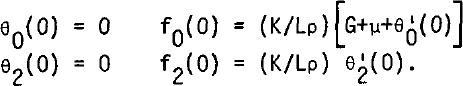
Our procedure computes successively θ₀, θ₂, η₀, η₂, f₂, f₀, according to the following equations:

(15)

The boundary conditions at the surface are:

(16)

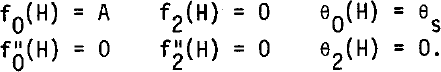
For a cold bottom:

(17)

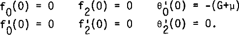
For a temperate bottom, L denoting the latent heat of ice:

(18)

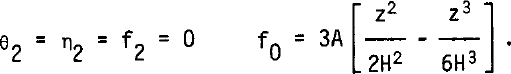
As starting values, the following ones, which satisfy the boundary conditions for the cold bottom case, but not all equations (15), are adopted:

(19)

If, during the computation, the temperature at the bottom reaches the melting point, the procedure switches to the one for a temperate bottom, and vice versa.

Results from the numerical model

Computation was done by a second-order finite-difference method with H = 3400, k = 36.8 - 0.09 θ m² a⁻¹, θ_s = -53.7°C (the actual surface temperature), -55°C or -60°C, and several realistic values for ϕ, A, G, k₁, k₃. Convergence was obtained after about ten iterations when ϕ was not too small. Velocities and temperatures are insensitive to the adopted value for ϕ, and to the value of k₃ in the range 0.2 - 2 m a⁻¹ bar⁻³ (the term k₃ ^τb⁵> is totally negligible). The influence of k₁ on the temperatures is also negligible. We give our results for k₁ = 0.6 m a⁻¹ bar⁻¹.

Three cases may occur, which are summarized on Figure 3. Either the bottom is temperate (T), or it is cold (C), or no steady state exists (0). In the last case, temperate bottom conditions lead to a cold bottom, and the reverse, indefinitely. Our interpretation is that the regime should be cyclical: sliding allows more advection of cold towards the bottom, and freezing. No-sliding lessens this advection, and then the melting point is reached and sliding appears.

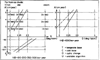
Fig.3 Results from numerical simulation (see text). Situation at the bottom, in the steady state, for different values of the accumulation A (in metres of ice), of the surface temperature es, and of the geothermal gradient G. Below each case, in brackets, value of h in Equation (1). Above, values of h given by (2), far from an ice divide.

Theoretical values of T'(z) for the steady state are given in Figure 2. They are more sensitive to accumulation than to the geothermal flux. In any case the steady state value for T" is larger than the actual one, which shows that the transient term Ṫ in Equation (3) cannot be neglected.

T(z) and θ(z) are plotted in Figure 4. It appears that Dansgaard and Johnsen's analytical expression for w (Equation (2)) is valid for the upper two thirds of the ice sheet. Values of parameter h will be found in Figure 3 (as well as those calculated from Lliboutry's formula which, as has already been said, is not valid at an ice divide).

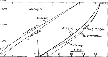
Fig.4 Left: vertical velocity w. Right: theoretical temperature profiles (steady state).

Calculation of the transient term in the temperature profile

Within the firn layer of a real ice sheet, changes in the surface temperature propagate downwards owing to thermal diffusion much more than to solid advection. Since at 10 m depth a mean annual temperature is reached, at the firn-ice limit, about 100 m deep, a mean secular temperature should be reached. Now, (at Dome C) about 2 ka are needed for firn to reach this depth.

The thermal diffusivity of snow or firn, whatever its density, is about 13 m² a⁻¹, one third of its value for ice (Lliboutry 1964: 394). Nevertheless, it has been measured under conditions when heat transit through the air phase comes only from molecular diffusion, ignoring any vertical motion of the air within the névé caused by atmospheric pressure changes or gusts of wind. Thus, the actual thermal diffusivity of firn is larger, and unknown.

For these reasons, it is impossible to-day to calculate transient temperature profiles within the firn, and we shall calculate transient temperatures below 100 m depth only. The precise phase lag between temperature oscillations at 100 m depth and at the surface (said to be of the order of one century) is unknown, as well as their damping. Only mean temperatures over one millenium or more will be significant.

At this large time scale, our model, in which the firn is replaced by an ice layer of the same weight, may be retained. To study how a perturbation in the surface temperature propagates downward with time, the values A = 37 mm a⁻¹ (the present accumulation), G = 0.0225 deg m⁻¹ and 1/ϕ = 300 bar a were adopted. This is a limiting case, where both conditions T_b = T_f and W_b = 0 are satisfied. The corresponding value of h is 300 m, approximately the one given by Lliboutry's formula.

The perturbation in the temperature is assumed not to change the flow, and so only remains a problem of heat diffusion in a moving medium. It was solved by a method indicated by Douglas and Jones (Remson and others 1971:98-101), which is a variant of the Crank-Nicholson method. Our program was tested by computing the temperatures in the case handled by Reference WhillansWhillans (1978) (although he adopts h = 0, the difference remains negligible in the upper layers). Our results are given in Figure 5. They show that, in the case of Dome C, the ice sheet still reacts to surface temperature changes during the Riss-Wiirm interglacial.

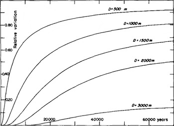
Fig.5 Response of the temperature within the ice sheet to a step at time zero, as temperature variation at the surface. A: 3.7 cm a⁻¹, G: 0.0225 deg m⁻¹.

After calculating the impulsive response, it was convolved with palaeotemperatures drawn from ¹⁸0 data (Lorius and others 1979). Their time scale is drawn from the rough expression (1) for the vertical velocity, with h = 0, w_s = -A, and A = 37 mm a⁻¹ down to 381 m depth (equivalent to 10.921 ka BP), A decreasing linearly from 37 to 27.8 between 381 and 510 m depth, and A = 27.8 mm a⁻¹ from 510 to 873 m depth (equivalent to from 15.516 to 31.956 ka BP).

This time scale may be improved by using our better calculation, but, since it has been fitted on well-dated climatic accidents, the correction would be negligible. In order to avoid any spurious effect, all the measured palaeotemperatures were used, not smoothed values. An important correction was made to account for the change in the 180 content of oceans during the glacial epoch.

Results are given on Figure 6. The theoretical Ṫ(z) has important fluctuations within the studied range of depth. The negative spike (-6.9 × 10⁻⁴ deg a⁻¹) at 150 m depth corresponds to the ending of the hypsithermai, the first maximum (1.3 × 10⁻⁴ deg a⁻¹) to its beginning, and the broader one (2.0 × 10⁻⁴ deg a⁻¹) around 1 000 m depth to the warming which ended the last ice age. The mean value of Ṫ(z) between 100 and 800 m depth (including all the negative spike) is found to be 0.38 × 10⁻⁴ deg a⁻¹. The mean value of Ṫ(z) between 230 m (when it becomes positive) and 800 m is found to be 1.02 × 10⁻⁴ deg a⁻¹

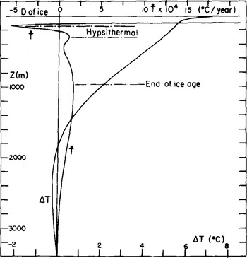
Fig.6 Theoretical values of the present, temperature variation ΔT and its time derivative Ṫ, as drawn from ¹⁸0 palaeotemperatures.

Estimation of Ḣ, and discussion

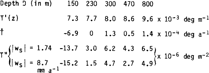
The mean value of Ṫ(z) in the bore hole is very poorly known, as a consequence of the strong variability of Ṫ(z) near the surface. The two above-mentioned values may be considered as lower and upper bounds. Let us use now relation (4), with k = 41.5 m² a⁻¹. Between 75 and 825 m depth, mean values of T' and T" are, respectively, 8.5 × 10⁻³ deg m⁻¹ and 4.0 × 10⁻⁶ deg m⁻¹. The resulting mean value for the vertical velocity is -7.5 to -15 mm a⁻¹.

This is the velocity at 450 m in depth, measured from the true snow surface. The ice equivalent surface is about 20 in lower. The vertical velocity at depth D is then:

(20)

It follows w_s = -17.4 to -8.7 mm a⁻¹

Dome C should have risen by 200 to 280 m during the last 10 ka. Velocities should be two to four times smaller than the balance velocities. As a consequence (which allows this fact to be discovered), the temperature profile is more linear than it would be in the steady state.

By adopting the values above for ws, the fluctuations in T"(z) can now be computed (Table II).

Table II PREDICTED VALUES OF T"(z)

Actual fluctuations of T", as estimated from Figure 2, are of the same order of magnitude as the computed ones, but the accuracy is insufficient to allow any significant check.