


Introduction
The huge ice masses caused by large grounded ice sheets result in depression of the Earth’s surface. This specific response of the planet is known as the isostatic response and in return acts on these ice sheets, and therefore has fully to be taken into account in any ice-sheet modelling attempt. Indeed, in the case of isostatic equilibrium, the Earth deflection can be as much as one-third of the ice thickness according to the hydrostatic approximation. It means a lowering of up to 1 km below the thickest parts of large ice sheets. One can easily realize the consequences of such a shift on the ice cap in terms of surface mass balance. Another crucial point lies in the specific geometry of accommodation in the vicinity of the ice-sheet margin, mainly controlled by the lithospheric elastic bending. The peripheral forebulge induced by the asthenospheric viscous outflow may also play a role beyond the grounded-ice limit. In the case of a marine ice sheet, such as in West Antarctica, an accurate parameterization of the bedrock elevation, in these sensitive areas seems crucial. It permits proper determination of the grounding-line migration according to the relative sea-level changes, and the consequent effects on the stability of the ice shelf (Huybrechts, 1990a, b, 1992; Le Meur and Huybrechts, 1996). Besides the effects of specific geometrical aspect, the lagged response of the Earth strongly influences the time-dependant behaviour of ice sheets. It is even generally argued that these ice-Earth processes would partly explain the characteristic 100 kyear period over which ice caps have regularly grown and decayed for the last 800 000 years. Nevertheless, as crucial as it may appear, the development of a realistic Earth model still encounters many difficulties. One of the most important points lies in the appropriate choice for a rheological law which must be sufficiently realistic, without being too complex to model. For that purpose, linear rheologies are particularly appreciated, since they allow model linear outputs with respect to the loading values, a crucial property for the convolution process of the Green functions. Section 1 explains the main reasons for using such rheologies and also to what extent these linear parameterizations can be simplified. The second major issue concerns the correct determination of the Earth parameters. Some of them are relatively well known from seismic data, such as the Hookean parameters and the density profile (Dwiezonsky and Anderson, 1981), whereas others remain uncertain such as the viscosity profile within the mantle. In order to cope with this problem, a calibration test on viscosity is carried out by matching the numerous data derived from Fennoscandia (sections 2 and 3). Finally, section 4 goes deeper into the results from the reference model that resulted from this study.
1 The Model Philosophy
1.1. The visco-elastic theory
Due to the large-scale displacements provided by the glacio-isostatic process, an accurate modelling of the Earth response under large ice sheets requires spherical models that take into account the whole planet (Peltier, 1974; Cathles, 1975; Lambeck and others, 1990; Spada and others, 1992). These kinds of model manage to reproduce correctly the displacement field (especially the deep part) and therefore can easily incorporate the complex interactions between this latter and the gravitational potential field (Bachus, 1967; Peltier, 1974). The four main parts generally adopted for the planet consist of an inner inviscid core surrounded by a viscous mantle (which is often split into an inner lower mantle and an outer upper one), and finally a peripheral elastic litho-sphere. Most of the deformation takes place in the mantle under the form of a visco-elastic flow (the use of this terminology will be clarified later on) and, to a lesser degree, in the lithosphere which essentially bends elastically. These preliminary considerations led to the now generally accepted family of self-gravitating spherical visco-elastic models (Peltier, 1974; Lambeck and others, 1990; Spada and others, 1992). The crucial issue is in fact the way the mantle rheology is treated. The two main questions are (i) whether one can consider the relation between stress and strain rate as linear, and (ii) how to deal with the deviations from the perfectly elastic behaviour for the short time-limit response (revealed by seismic surface-wave attenuation). As regards the long time limit (for times in excess of several hundred years), the mantle is subject to a steady-state viscous flow that some laboratory experiments have tried to reproduce (Kohlstedt and Goetze, 1974; Durham and Goetze, 1977). Unfortunately, these results have suggested a non-linear flow law, at least at the strain-rate characteristics of laboratory-induced creeps (10−6 s−1). However, as argued by Peltier (1982), these rates are far higher than those encountered in the mantle (10−16 s−1), and the corresponding stress levels would favour grain-boundary processes instead of the single-crystal deformation obtained by experiments. Some other studies (Twiss, 1976; Berckhemer and others, 1979; Brethau and others, 1979; Greenwood and others, 1980) even suggest that this grain-boundary creep process might obey a linear constitutive relation. As regards short time-scale behaviour, it seems from recent work in seismology that this anelasticity also fits in the framework of a linear relation.
Finally, Peltier and others (1981) have even claimed that there exists a single linear model capable of continuously describing the whole geodynamic time spectrum, and especially the transition from the short-term anelasticity to the long-term steady-state viscous flow. The so called “generalized Burgers body”, when expressed under its simplified form (the Burgers body), still yields a rather complex stress-strain relation. However, Peltier (1982) first showed that, when one tries to infer the characteristic parameters of such a model in order to match the quality factors, it appears that in the short-time limit, the deviations from a perfectly elastic behaviour are not very large. Secondly, the steady viscous flow that rapidly takes over and becomes the predominant deformation process in the postglacial rebound, can easily be treated with a simple viscous Newtonian stress-strain relation. On the basis of these two considerations, and following most of the self-gravitating spherical visco-elastic models (Peltier, 1974; Lambeck and others, 1990; Spada and others, 1992), the rheological body used in this study has been “reduced” to a simpler Maxwell body. It consists of a spring and a dashpot in series. Only three parameters are nccessary to characterize entirely the mechanical behaviour, namely λ and μ, the two conventional Lamé constants for a Hookean elastic solid, and v, the viscosity governing the strain rate for the viscous flow. For a Maxwell body, the linear combination between the stress tensor τ kl , the strain tensor e kl and their respective time derivatives (dotted tensors) reads

In the Laplace-transform domain, where the tensors are now expressed in terms of their Laplace transforms, according to

the constitutive relation in Equation (1) reduces to
which is exactly that for a Hookean solid, but with the coefficients λ and μ now functions of the laplace variable s according to

This formalism illustrates the correspondence principle (Peltier, 1974), which states that it becomes possible, by shifting to the Laplace-transform domain, to reduce any linear rheology to a simple elastic Hookean treatment. To understand this approach, s and μ/ν must be interpreted as inverse times, then the value s = ¼/½ = −1/T
m clearly appears to be singular and is the inverse of the so called “Maxwell time T
m. It means that for short time-scales corresponding to |s| » μ/ν the terms λ(s) and μ(s), respectively, tend towards the conventional Lamé parameters λ and μ, indicating a Hookean elastic behaviour. Conversely, for low values of |s| corresponding to time values far greater than the Maxwell time (t » T
m), λ(s) and μ(s), respectively, tend towards K and vs. In the time domain, this yields a stress-strain relation characteristic of an incompressible viscous fluid, that is: τ
kl
= Kd
ii
δ
kl
+ ![]() . The full visco-elastic treatment allowed by this principle comes from the fact that the entire frequency s-spectrum is considered from the elastic limit to the large time-scale viscous flow. The time-dependent solution is obtained from the Laplace inversion of the s-dependent solution of the equivalent elastic problem. This method is fundamentally different from that employed by Cathles (1975), which treats the viscous and elastic systems of equations separately at each time step and adds them to approximate the total displacement. A paper by Wu (1992) clearly shows that this latter approach gives poor results compared to those from the correspondence principle, as far as the mantle is supposed to be visco-elastic.
. The full visco-elastic treatment allowed by this principle comes from the fact that the entire frequency s-spectrum is considered from the elastic limit to the large time-scale viscous flow. The time-dependent solution is obtained from the Laplace inversion of the s-dependent solution of the equivalent elastic problem. This method is fundamentally different from that employed by Cathles (1975), which treats the viscous and elastic systems of equations separately at each time step and adds them to approximate the total displacement. A paper by Wu (1992) clearly shows that this latter approach gives poor results compared to those from the correspondence principle, as far as the mantle is supposed to be visco-elastic.
1.2. The unit model
We are now concerned with the elastic-equivalent problem of the response to the surface loading for a self-gravitating spherical Earth. The appropriate equations for momentum conservation, gravitational and density perturbations have been linearized with respect to small perturbations from a hydrostatic initial equilibrium (Bachus, 1967), The unit-impulse point load and the ensuing symmetry of the problem are particularly suitable for a spherical surface harmonical treatment. Therefore, the new spectral variables depend only on the radius within the Earth. The linearity in both the stress–strain relation and the elastic equations allow the superposition of each harmonic contribution in the final solution. For instance, the solution displacement vector u and the solution gravitational potential perturbation scalar φ reads

where er is a radial unit vector. eθ a tangential one. r the radial distance from the centre of the Earth and Pn the nth degree Legendre polynomial. Then Un , Vn , Φ n are the corresponding spectral amplitude solutions for the radial and tangential displacements and the gravitational potential perturbation, respectively, in response to the nth degree component of the load.
In the spectral domain, the expression of the quasi-static elastic equations and the stress–strain relation gives a system of six first-order ordinary differential equations which are solved numerically with the appropriate boundary conditions at the two end points of the domain. Then, a normal-mode method for inverting the Laplace transform (Peltier, 1985) yields the time dependent impulse response under the form of an instantaneous response  (the superscript E denoting the elastic instantaneous contribution) followed by several viscous decay modes. So the Love number Yn(r, t) or, in other words, the contribution of the nth harmonic degree takes the form

where the snj (j = 1 to N) represent N discrete values of the Laplace variable s and are the inverse characteristic accommodation time-scales of each of the N viscous modes, and Rn, j the corresponding amplitude. Recall that we are in the transformed space and therefore dealing with spectral variables like Yn(r, t); we still have to recover the colatitude-dependence θ by summing these variables with the associated Legendre polynomial according to Equation (5).
The procedure followed up to now is virtually the same for most of the self-gravitating visco-elastic spherical models and leads to the computation of the Green function. As this Green function represents the Earth response to a unit-impulse load, it is in fact a direct consequence of the structure of the planet assumed by the model. Therefore, the difference between these models will essentially come from the different ways of accounting for this structure and from the different numerical treatments used for solving the ordinary differential equations system. One specific feature of the present model lies in a computation, for seismic data, of some Earth properties like the elastic shear and compression moduli, the density and the gravitational acceleration within each of the main Earth domains. Only the viscosity profile, which remains the most uncertain, is kept constant within two layers (lower and upper mantle). Although this method yields the same major discontinuities in the density and viscosity profiles at the end points of the domains as those based on successive layers of uniform parameters (Spada and others, 1992), the ensuing extra viscous modes exhibit different characteristics (amplitude and time constant). Finally, the total response to any realistic load will come from the convolution of this “unit” Green function Y(a, θ, t) at the surface (a is the Earth’s radius) with the space–time history of that load (Peltier, 1974], From there one can distinguish two ways of application fur such a model. On the one hand, the model can be forced by a prescribed glacial scenario to match the time-dependent Earth response as in the present study. On the other one, the model can also be fully coupled with an ice-sheet model in order to take into account the bedrock response in the ice dynamics (Le Metur and Huybrechts, 1996). In order to account properly for this bedrock effect, the isostatic response has to be computed as often as possible for the new bedrock profile to be re-inserted in the ice model and the ice-flow pattern to be calculated accordingly. It therefore implies many calls to an “isostatic sub-routine” especially for long-term palaeoclimate simulations and that makes the use of the Green function very suitable since the “coupling” eventually reduces to a convolution process.
2 Coupling of the Green Function with a Glacial Scenario Over Fennoscandia
2.1. The loading scenario
As we are concerned with postglacial rebound, the loading scenario with which the impulse Green function is to be convoluted essentially spans the last great deglaciation period, that is between 18 000 years and 8000 years BP. We did not apply the exact estimate of the Fennoscandian ice-sheet maximum extent at the Last Glacial Maximum (LGM) about 18 000 years ago compiled by Andersen in Denton and Hughes (1981). Because it is now generally believed that this reconstruction gives exaggerated thicknesses (Nesje and Dahl, 1990; Fjeldskaar, 1994), a global thickening of about 500 m has been applied all over the ice sheet to yield a more realistic initial configuration (Fig. 1). From there, the specific deglaciation chronology was derived from a space–time interpolation of a 5° by 5° gridded reconstruction (ICE-1; Peltier and Andrews, I976), giving the deglaciation profile every 2000 years. By successively applying these interpolated ice-sheet changes every 1000 years to our initial maximum configuration (which first has to be digitized on our 50 km by 50 km spatial grid), we finally obtained the required glacial scenario (see snapshots in Figures 1, 2 and 3). As well as the changes in ice thickness the sea-level variations have to be integrated and substantially contribute to the isostalic response not only below the sea but also far inland (see the regional aspect of the Earth response; Le Meur and Huybrechts, 1996). This hydro-isostatic effect is all the more important since mean sea level has undergone strong variations when the Northern Hemisphere large ice sheets suddenly disintegrated during the deglaciation period mentioned above. Indeed, mean sea level is supposed to have risen by about 130 m between the IGM when northern ice sheets were at their paroxysm and approximately 8000 years ago when the last ice melted, to finally reach a mean level close to the present one (Figs 1–3). The geoidal eustatism has been neglected in the hydro-isostatic component of the total Earth response in the sense that we have assumed a uniform ocean filling as the Northern Hemisphere ice sheets disintegrated. However, such a contribution must be negligible in terms of Earth surface displacements and is essentially worth accounting when modelling accurate sea-level patterns.

Fig. 1. The initial ice-loading configuration used in the present study for the Last Glacial Maximum 18 000 years ago. Contours are given every 250 m end the maximum thickness is 2640 m. Ice loading over Iceland is not considered. The white fringe represents the aerially exposed areas as a consequence of the sea-level lowering of 130 m for that time.
2.2. The memory effect and the impacts of initial conditions
The philosophy of the unit model is to provide an impulse Green function like that depicted in Equation (6) as the response to an impulse-unit load which can be represented as a 1 kg needle pressed on to the Earth and instantaneously removed. The response to any realistic load will come from a double space–time convolution of this unit response with the history of that load. For the sake of simplicity, and to illustrate our present purpose, we can now consider a point load characterized by its time-dependent history, say H(t). If Y(r, t) in Equation (6) represents the Green function for the surface displacement, for instance, then the time-dependent surface displacement DISP(t) induced by that load is given by

where a is the Earth’s radius. Contrary to the impulse ease depicted in liquation (6), where the response is instantaneously given by summing the different modes, we see that in the present ease one has to integrate the contribution of all the previous loads prevailing before the time t we consider. This illustrates what we call the memory effect. In practice, because of the exponentially decaying response, and according to the respective amplitudes Rn, j and characteristic time constants Tn, j = −1/s n, j for each viscous model (see Equation (6)), more than 99.9% of the response is accounted for when this memory period is limited to 30 kyears. This memory effect emphasizes the problem of the correct choice for initial conditions, especially in the present case where only a few indications of the ice-sheet behaviour before the LGM are available. According to our memory period, one should theoretically know the glacial scenario from 48 000 years BP to restore properly the Earth response at around the LGM. Regarding present-day patterns, the loading history since 30 000 years BP has to be known and still includes periods before the LGM. Therefore, the main issue lies in the correct determination of the glacial scenario prior to the LGM, a question that has always been a subject of much debate. We should nevertheless keep in mind that more than 90% of the response is already achieved in 15 000 years. Because the uncertainty essentially concerns the duration of the maximum ice extent before 18000 years ago, one can expect only small changes depending on the scenario chosen for that period, as revealed by the following experiment.

Fig. 2. The glacial scenario at 14 kye\zetaars BP. The corresponding sea-level drop is 106 m.

Fig. 3. The glacial scenario at 10 kyears BP. The corresponding sea-level drop is 27 m.

Fig. 4. The two different scenarios tested in the sensitivity to initial conditions in terms of total ice volume. For the loading-scenario B, the ice thicknesses before the LGM (left of the vertical dashed line) cue deduced from that for the LGM with a weighting factor between 0.6 and 1 to match the reconstruction from Baumann and others (1995).
In this study, two different scenarios are tested (Fig. 4). The first (A) considers a constant LGM ice-maximum load so that a steady state is reached at 18 kyears BP, whereas the second (B) supposes ice-load fluctuations that have been deduced from an ice-sheet extent reconstruction of Baumann and others (1995). The corresponding Earth response is depicted on Figure 5 under the form of three deflection profiles along a southwest northeast transect (defined later on but observable in figures 6 and 7, and 10–14) at 18 kyears BP, 8 kyears BP and at the present time, respectively. As initially guessed, the difference in the results is only significant for the LGM profile (less than 20 m at the centre of the depression) and vanishes very fast as time goes on. The convergence is so fast that the results for periods around the present time can almost be considered as independent of the scenario prior to the LGM. Therefore, an initial bedrock configuration in steady state with the LGM maximum load can reasonably be used in the framework of this paper.

Fig. 5. Deflection profiles along the transect for the initial condition test. A and B stand for the corresponding scenarios whereas −18, −8 and 0 stand for 18 kyears BP, 8 kyears BP and present, respectively.
2.3. The interest of modelling the Earth response over Fennoscandia
Fennoscandia has been an area of great interest for postglacial rebound studies for the past decades and, as such, has been subject to many field-measurement campaigns. The main reason is the fact that this area has not entirely recovered the steady-state surface geometry corresponding to the present ice-free conditions. Ii means that the Earth still experiences the influence of the past ice-loading events with a still existing depression, a feature that illustrates the “memory effect”. The rate at which this depression is still rising today, as well as the free-air gravity anomaly resulting from the induced lack of matter, have been recorded during the many campaigns mentioned above. Since they are available, these data, when correctly reproduced by isostatic rebound models, provide an opportunity to assess the main Earth parameters such as the lithospheric thickness or the viscosity profile within the mantle. Some recent studies (Lambeck and others, 1990; Mitrovica and Peltier, 1993; etc.) reveal a consensus as regards the ranges within which the different parameters obtained are varying. The bounds for the Earth parameters in the following calibration study will be fixed accordingly (see Table 1). The second main advantage of studying Fennoscandia lies in the good knowledge of the formerb ice-sheet maximum extension deduced from accurate mapping of the peripheral moraines (Denton and Hughes, 1981), or from the information content of ice-rafted detritus (Baumann and others, 1995), and also in the numerous attempts in reconstructing the ice-sheet disintegration chronology. As the glacial scenario is the only input for the unit model according to Equation (7), one should note the importance for such an input to be as realistic as possible, especially for the sensitivity study that follows.
3 Calibration of the Model According to Viscosity
3.1. The sensitive parameters for the model
As a preliminary remark, it should he stressed that Earth models are not only sensitive to the classical parameters such as viscosity but they also depend on the way the rheology of the planet is treated. However, for the reasons mentioned in section 1.1, the flow law will remain that of a Maxwell body throughout this study, although some tests on different rheologies might improve the model accuracy. Therefore, we will essentially focus on the different combinations of viscosity values within the two layers of the mantle (table 1). No tests have been carried out varying the lithospheric thickness since this parameter essentially controls the final shape of the degree of depression (essentially at the margins of the ice sheet) but not its chronology as the viscosity does. The second reason derives from the general agreement in the literature for a mean value of about 100 km (Lambeck and others, 1990; Mitrovica and Peltier, 1993), which is in line with geodynamical evidence (plate-tectonics theory), at least for stable ancient shields such as Fennoscandia. The lithospheric thickness is nevertheless crucial when one requires an accurate geometrical treatment close to the grounding line, when dealing with the stability of marine ice sheets (Le Meur and Huybrechts, 1996). Finally, it should be mentioned that the lithosphere may undergo quite drastic thickness changes in other locations such as across orogenic belts (Transantarctic Mountains) or close to ocean ridges (Iceland).
Table 1. Viscosity values for the six first runs in Pa s. The top row gives the upper-mantle viscosity, whereas the left column gives the lower mantle one. One can notice that the lower mantle is always taken to be more viscous than the upper one except for run 4


Fig. 7. Map of a 4° by 8° smoothed free-air gravity anomaly in mgal over Fennoscandia (from Bailing, 1980). These values have to be lowered by about 10 mgal in order to provide relevant equivalent remaining displacements.

Fig. 6. Map of the present-day rate of uplift over Fennoscandia (from Bailing, 1980). The contours are in mm a−1 and refer to the mean sea level. Absolute vertical velocities are obtained in adding the present-day eustatic component (about 1 mm a−1) to these values. The southwest–northeast transect for the sensitivity test has been outlined.

Fig. 8. Modelled rates of uplift for runs 1 to 7 along the southwest—northeast transect. The expected maximum value of 10 mm a−1 value is outlined.
3.2. The validation criteria
Before starting the experiments, a validation criterion had to be defined on the basis of the present-day rate of uplift (Fig. 6) and gravity anomaly (Fig. 7) compiled by Bailing (1980). All the simulations from this first set of experiments gave a modelled present-day rate of uplift quite similar in shape but with different values. So an appropriate southwest northeast transect (depicted in figs 6 and 7, and 10–14) passing through the area of maximum uplift (Gulf of Bothnia) appeared to be adequate for comparing the different nuts. Indeed, they all show different rate profiles (Fig. 8) and the agreement with the maximum observed value (depicted by the horizontal 10 mm a−1 line) provides a first criterion. One can notice that 10 mm a−1 is somewhat larger than what can be deduced from Figure 6. The reason is that the maximum value at the centre of the ellipse must be close to 9 mm a−1 and the levelling has been performed by referring to mean sea level which is assumed to be rising by about 1 mm year−1 at the present time (Fjeldskaar, 1994). The second criterion does not derive from a direct comparison of the gravity fields, because the data are less smoothed as a consequence of local geological heterogeneity. They are also globally biased according to Bailing (1980). Anyway, a map such as Figure 7 is still interpretable once the geological perturbation has been roughly estimated and corrected for and once a global lowering of about 10 mgal has been applied. It is now generally believed that the pure isostatic component of the free-air gravity anomaly reaches a maximum of about −15 to −20 mgal over the Gulf of Bothnia. This free-air gravity anomaly is directly connected to the deviations of the present surface height from the ice-free steady state one. Indeed, there is a simple formula relating the remaining displacements to this anomaly (Lliboutry, 1965), which is

with h the displacement in metres. △g the anomaly in mgal, ρa the asthenospheric density and G the gravitational constant. Then we can derive our second criterion by checking the remaining displacements along the same transect (Fig. 9), especially with the minimum value in the vicinity of the Gulf of Bothnia. According to Equation (8), this value should lie between about 100 and 150 m.

Fig. 9. Deviation from steady state at present in terms of surface displacements along the transect for runs 1 to 7. These distances can also be interpreted as the expected displacements to come in the future before the surface reaches the ice-free condition steady state (flat surface).
3.3. Results of the experiments
The calibration of the model has been carried out in two steps. A first set of six simulations has been performed according to Table 1, where the viscosity values were chosen without any a priori but just in order to range within commonly accepted bounds. Then, on the basis of these results, it became possible to fit optimal viscosities for both the lower and upper mantle in a final realistic run (run 7) to which we are able to refer in future. The results from all these seven runs are depicted in Figure 8 in terms of present-day rate of uplift and in Figure 9 in terms of the remaining displacements needed to reach a steady state. Disregarding run 7, inspection of figures 8 and 9 reveals the main postglacial time dependent behaviour as a function of a mean viscosity value representative of the whole mantle (at this stage, no distinction between the lower and upper mantle wall be considered in the interpretation). Indeed, runs 1 and 2 are characterized by the highest global viscosity values (see Table 1) and show higher uplift rates and remaining displacements from a second group made of runs 5 and 6 (lowest global viscosity values). As surprising as they may seem in a first instance, these results are somewhat consistent in the sense that for the high-viscosity group the equilibrium state is still far off, whereas for the low-viscosity one a steady state has almost entirely recovered. Then, the higher uplift rates also become explicable as they appear to be more sensitive to the state of imbalance than to the viscosity itself. Unfortunately, none of the runs carried out there has given entirely satisfactory results, since each of them does not fit at least one of the two sets of data. However, these preliminary results can help in a refinement of the viscosity values with a final simulation. The remaining displacements seem to favour a lower mantle viscosity between that for runs 1 and 2(2.5 × 10²¹ Pa s) and that for runs 5 and 6 (1.0 × 10²¹ Pa s), whereas matching of the correct late of uplift requires a parameterization close to that for run 5. Finally, the supposed reference model was run with a lower mantle viscosity of 1.5 × 10²¹ Pa s and an upper mantle viscosity of 7.5 × 10²⁰ Pa s. Despite the fact that run 7 does not strictly match any of the two criteria, it nevertheless gives the best global fit with a maximum uplift of 11.5 mm a−1 and a maximum remaining depression of 72 m along the transect.

Fig. 10. Steady-state response of the reference model in terms of surface displacements in m for the LGM, 18 kyears ago. The consequences of the sea-level lowering (130 m) are depicted as on Figures 1–3.
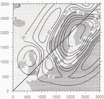
Fig. 11. The same as Figure 10 but for 8 kyears BP and with a corresponding sea-level retreat of 7 m.

Fig. 12. Displacement pattern for the present day in m. These values can also be interpreted as the remaining displacements before the model recovers a steady state (flat surface), that is, in the present case, in about 23 000 rears, or in other words, 30 000 years after the last crystal of ice melted (memory effect).
4 Illustration of the Main Postglacial Rebound Features with the Reference Model
4.1. Surface-displacement patterns
Figures 10–12 show the different surface-deformation patterns at 18 kyears, 8 kyears BP and at the present time for the reference model in response to the glacial scenario described above (Figs. 1–3). The first characteristic geometrical feature comes from the lithosphere, which bends like an elastic plate under the load and gives rise to deviations to an idealized hydrostatic profile (Le Meur and Huybrechts, 1996), As a consequence, the maximum depression is reduced and only readies 600 m in a steady state at 18 kyears BP (Fig. 10) instead of about the 800 m that a hydrostatic calculation would predict, according to the maximum ice thickness (2640 m). On the other hand, this depression expands further from the ice-sheet margin (see Figure 10; for instance, the ice-free area between Norway and the British Isles), so that the total asthenospheric displaced volume below the lithosphere is the same as it would be using the hydrostatic solution. The second noticeable geometrical feature is a direct expression of the slow creep processes taking place within the underlying mantle. There, the substratum flows out under the pressure exerted by the lithosphere and creates a peripheral forebulge. This forebulge, whose height is generally about one-tenth of the central depression, often interfers with the outermost part of the depression due to the lithosphere and makes these two structures sometimes difficult to identify (Le Meur, in press). Another point worth noting from Figures 10–12 is the specific timing of the Earth response to an ice sheet. Indeed, among the different geodynamical processes that load the Earth surface, ice sheets seem to be the only ones able to provide sufficiently fast-varying loads to induce a transient response from the mantle. In other words, during the rapid decay of the Fennoscandian ice sheet, the planet does not have time to accommodate entirely a prescribed ice thickness before the latter evolves to another value. As a consequence, at 8 kyears BP (Fig. 11), the central depression is still more than 300 m deep, despite an equilibrium value of less than 160 m according to a maximum ice thickness of about 500 m. This characteristic transient isostatic rebound is, of course, remarkably illustrated by the present-day imbalance (Fig. 12). It means that the Earth has not yet recovered the equilibrium surface corresponding to the present-day zero load (a flat surface in the present case), even if this load has remained constant for the past 7000 years. This justifies the memory effect (see above) and especially values of the order of 104 years for the time-integration period.
4.2. Uplift and free-air gravity anomaly patterns
Despite slightly different values, the present-day rate of uplift given by the model is in quite good agreement with the data as regards the global shape (figs 6 and 13). The elliptical shape is correctly reproduced as well as the areas of rising and sinking delimited by the zero contour, which follows the Norwegian coast and crosses Denmark and the Baltic Sea. Unfortunately, the data from Bailing do not provide information farther away, to which the model results could be compared. However, some sea-level measurements along the North Sea coast gave, according to Lliboutry (1965), a rise of 37 cm per 100 years at the mouth of the River Weser (northern Germany) and of 20 cm per 100 years in Lubeck (Netherlands). The assumed eustatic component being 10 cm per 100 years, the deduced rate of sinking becomes close to the model outputs (see the −2 mm a−1 and −3 mm a−1 contours over these areas). As regards the free-air gravity anomaly pattern (Fig. 14), the comparison with the direct measurements is not straightforward for the reasons previously mentioned. It is nevertheless possible to check whether these results are consistent with the other model outputs. As the free-air gravity anomaly is connected to the remaining displacements, the good correlation with the uplift becomes obvious from figures 13 and 14 with similar respective depressed and rising areas. Additionally, the minimum anomaly of −12 mgal suggests (according to Equation (8)) a remaining displacement of about 87 m, in somewhat good agreement with the actual maximum depression value of 77 m given by the model (not exactly on the transect).

Fig. 13. Map of the present-day rate of Uplift in mm a−1 for the reference run.

Fig. 14. Map of the free-air gravity anomaly in mgal for the reference run.
Conclusion
Earth models are interesting for two main purposes. On the one hand, they can help in inferring the most poorly constrained parameters for the planet such as the mantle viscosity. On the other hand, they can be fully coupled with the now available three-dimensional ice-sheet models to account for the isostatic impact on the ice behaviour (Le Meur and Huybrechts, 1996). In order to carry out this last task with success, one has to be sure the isostatic model is sufficiently realistic. Unfortunately, current ice sheets do not provide any efficient way of testing the Earth contribution (see the paper by Le Meur and Huybrechts, 1996). Only recently, ice-free areas like North America or Fennoscandia have offered the possibility of time-lagged isostatic effects, with which one may check the model validity. As this study tends to show, the model is sensitive to both the Earth parameters and the assumptions as regards the rheology, and making a correct sensitivity test is very difficult. In fact, we should need another independent way of checking these parameters and also a more confident former ice-sheet history. However, the fact that the model seems able to more or less reproduce several different isostatic features and measured data make the full coupling with an ice-sheet model worth performing. The expected results should therefore be at least as good as those obtained using simpler and obviously less realistic bedrock parameterizations.
Acknowledgements
The author thanks the EISMINT initiative for having led fruitful workshops and funded several participations, during which much has been learnt about ice-sheet modelling. This work has been undertaken wish the financial support and the collaboration of B.R.G.M. — Département Géologie, Service Risques Naturels et Géodynamique Récente, under a grant from the ANDRA, and largely benefited from the excellent calculation facilities provided by the Alfred-Wegener-Institut (Germany). The author would also like to thank R. C. H. Hindmarsh for his help in the final editing of this paper.


